Download

1 / 22
220 likes | 240 Vues
Revamped planning support system for water management projects, linking database information, adding new substances, analyzing emissions, and integrating source data. Manage resources efficiently with improved tools and interfaces.

E N D
WEISS Planning Support System • Revised by Randbee Consultants for the WaterInnEU Project
Opening an existingWEISS project • We open the file Flanders.ini; • The project file is linked to a Microsoft access Database were all the information and data are stored into Hint: Open the Flanders.ini file with a block note, you will see the linked Database and the extent of the region map.
Adding the new substances Hint: If the Sum box isselected, you can view the results for the sum of all substances within that substance group. This is very useful for figure out the cumulative effects of the pollutant. • The substance list can be viewed in the tools group Emissions • For each group, you can assign the symbol and the name • There is the possibility to add the CAS number.
Addingsource • Here you can add: • Point sources (Import point sources…) • Diffuse sources (Import Estimation…) Hint: Diffuse sources are estimated with the emission factors and the emission explanatory variables. Important: these files MUST be in the CSV format.
Addingsource For the VOLVO CARS GENT point source we can see the emissions on surface water (Oppw). Hint: RIO means sewer discharger. Oppwmeans surface water discharger. The sectors and the sources are built with a hierarchical path: You have the possibility to create 4 levels at least
For a Source you can consult the flow chart to better understand how the gross emission are computed for a substance. For instance, let’s take a look to the zinc emission of the point source manufacturing of vehicles and let’s make the summary of all the emissions for each source: the result is the gross emission on the flow chart. Point sources Measurement of point source for manufacturing of vehicles – point source Pbt = 0 + 1125.2478 + 0 + 179.932858 + 259.557138 =1564.737796
Point sources We can do the same balance to better understand the substance’s sub-divionson the flow chart. For instance, the emissions of zinc for manufacturing of vehicles point source are split on RIO discharge and Oppw discharge. On the bottom left, you can see the balance for the partition of the emission. RIO Oppw Oppw zinc total emission 58037.69+10592.3+8590.53=77220.53 RIO zinc total emission 79006.124+27317.92=106324.044
Diffuse sources: Pathway, emission factor, Efficiency IWWT and rain sensibility • The Pathway is the way the pollutants reach the water body; • On the box in red you can see the four way of the path: Water, Surface, Drain, Loss; • Their sum is always 100. • The emission factor is expressed in g/cm for each substance; • The Efficiency IWWT is the performance of the waste water treatment platform to reduce the substance; • The Rain sensitivity is the range of the substance is linked to the rainfall.
Diffuse sources: EmissionExplanatoryVariable, EEV The emission explanatory Variable, EEV, is generally a GIS layer with geographic information and values information about the diffuse sources. (For more information about that, take a look to the theoretical presentation or read the Manual). After map (ASCII format) EEV uploaded, you will click on compute and after that you will create a map (take a look to the Figure above. This is the result for the computation of the EEV about the number of kilometer travelled by car on provincial roads. In other hands they have spatial information about the unit which the emission factor is referred to.
Add the year 2012 in WEISS and import the list of E-PRTR point sources of 2012 • We create a new version clicking on “New version…” based on 2010_a. • We do this after have locked the version 2010_a so the name must be 2010_a*. • After that, we can add the point source E-PRTR associated to 2012. To do this we consider diffuse source the same of 2010. Version 2012_a, SlachthuisVanlommel is not long in the list NOTE: Version 2010_a* apperslike that because it is locked.
Add new EEV for the 2012_a version • When you add a new EEV it’s important define: • The dimension • The unit • The algorithm that will be used • add: • The ascii map or the shape file • The optional attribute table linked to the map with the spatial information and the value.
Add new EEV for the 2012_a version For instance, for the water usage trade EEV we use the lu50m.asc as ancillary map and to apply the multi-resolution dasymetric mapping algorithm we use the weight written on the column named SS611 stored on the LANDUSE.DBF attribute table. HINT: The file .dbf can be opened with excel and you can read it. (take a look to the figure on the left) • Ancillary map: • Land use with resolution of 50 m.
Computation The calculations are carried out with the Compute tool You must specify: • The substance • The source or the sector • The version of the data file. If you check “Write ASCII map”, WEISS will generate for all maps computed an ascii version alongside the internal digital format.
Viewingresults On the analysis box you can click the “Flow chart” tool. Clicking on the blue box you can see the correlated map for that particular node. For instance, in this case we’ve chosen to view the gross emission to water map for the copper emission produced by seagoing vessels.
Viewingresults: choroplethmap and overlay WEISS has the possibility to show the results on a choropleth map and also to use a map for the overlay in the visualization. On the Map catalogue windows you can add the map for the Areal subdivisions and for the overlay For example, here you can see the choropleth map for the copper gross emission for the seagoing vessels with the overlay of the municipality shape.
Viewingresults: choroplethmap and overlay • The choropleth map for the copper gross emission for the seagoing vessels is generated using ports.asc • At the begin, the emission factor for that source is 300 g/number of moored seagoing vessel. • The EF is after multiplied for the Leaching antifouling seagoing vessels EEV with the unit of “number of vessels”. You can open the file where these information are stored: it’s called “eev_moored_seaships.dbf”. We can read the port’s name called NAAM in the table and the number of vessels in the column J2005. • Important: The choroplethmapwesawbeforewasespressed in g.
Viewing results: customizing the map legend • We can customize our map and its legend as we want. • Weiss gives us the possibility to edit them in this way: • The first thing to do [1] is clicking on “Generate class bounds…”. You can modify the legend and customize your scale as you want. Clicking on “Find best scale”, WEISS will search for the best scale for that type of map. • After that we click on “Generate labels…” [2] • And in the end we click on “Generate colours…” [3] You can customize the colors of the legend as you prefer. 3 2 1
Viewing results: Flow chart, domesticwaste water emission for zinc It is interesting to play with the value of each node in the flow chart. For example we did a simple balance about the substance reduction made by the waste water treatment platform. • Reduction of urban WWTP: 74,52% • Input pollutant 3524453.68 g • Removed pollutant 2626525.37 g • Output pollutant 897928.33 g • Reduction of individual WWTP: 50% • Input pollutant 397674.75 g • Removed pollutant 198837.38 g • Output pollutant 1998838.38 g
Viewing results: Top 10 emissions The Top 10 tool allows you to gain an insight, via a table and bar charts, into the major emission sources in the study area. • This is a classification about the source of the net emission of copper to the water surface. • The main source of gross emission to water is the domestic waste water. The quantities is reduced by WWTP. • Gross Emission to water for subsubsector expressed in ton. • Net emission to water for subsector expressed in ton.
Viewing results: Gross/Net emissions In the Gross/net tool, the gross emissions, the net emissions and the ratio of both are shown in tabular form for a substance-source/sub-sector/sector combination selected.
Viewing results: Net emissions Here you can visualize the net emission to water on a pie chart. You can customize the unit which the value will be shown, the subsector, the source and the zone.
Viewing results: Waste Water treatment Platform, WWTP • Here you can validate your modelling. • The measured influents are the truth and they are compared with the modelled influent. • The different between the measured influent and the modelled influent is the unexplained and it’s also evaluated as a ratio of the measured quantities.