S ervice A ggregated L inked S equential A ctivities
190 likes | 318 Vues
S ervice A ggregated L inked S equential A ctivities. S A L S A Team Geoffrey Fox Xiaohong Qiu Seung-Hee Bae Huapeng Yuan Indiana University Technology Collaboration George Chrysanthakopoulos Henrik Frystyk Nielsen Microsoft Application Collaboration

S ervice A ggregated L inked S equential A ctivities
E N D
Presentation Transcript
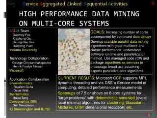
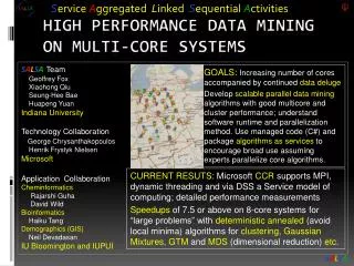
Service Aggregated Linked Sequential Activities SALSATeam Geoffrey Fox Xiaohong Qiu Seung-Hee Bae Huapeng Yuan Indiana University Technology Collaboration George Chrysanthakopoulos Henrik Frystyk Nielsen Microsoft Application Collaboration Cheminformatics Rajarshi Guha David Wild Bioinformatics Haiku Tang Demographics (GIS) Neil Devadasan IU Bloomington and IUPUI GOALS:Increasing number of cores accompanied by continueddata deluge Develop scalable parallel data mining algorithms with good multicore and cluster performance; understand software runtime and parallelization method. Use managed code (C#) and packagealgorithms as services to encourage broad use assuming experts parallelize core algorithms. CURRENT RESUTS: Microsoft CCR supports MPI, dynamic threading and via DSS a Service model of computing; detailed performance measurements Speedups of 7.5 or above on 8-core systems for “large problems” with deterministic annealed (avoid local minima) algorithms forclustering, Gaussian Mixtures, GTM and MDS (dimensional reduction)etc. SALSA
General Problem Classes N data points X(x) in D dimensional space OR points with dissimilarity ijdefined between them • Unsupervised Modeling • Find clusters without prejudice • Model distribution as clusters formed from Gaussian distributions with general shape • Both can use multi-resolution annealing • Dimensional Reduction/Embedding • Given vectors, map into lower dimension space “preserving topology” for visualization: SOM and GTM • Given ijassociate data points with vectors in a Euclidean space with Euclidean distance approximately ij: MDS (can anneal) and Random Projection Data Parallel over N data points X(x) SALSA
Deterministic Annealing • Minimize Free Energy F = E-TS where E objective function (energy) and S entropy. • Reduce temperature T logarithmically; T= is dominated by Entropy, T small by objective function • S regularizes E in a natural fashion • In simulated annealing, use Monte Carlo but in deterministic annealing, use mean field averages • <F> = exp(-E0/T) F over the Gibbs distribution P0 = exp(-E0/T) using an energy function E0 similar to E but for which integrals can be calculated • E0 = E for clustering and related problems • General simple choice is E0 = (xi - i)2where xi parameters to be annealed • E.g. MDS has quartic E and replace this by quadratic E0
N data points E(x) in D dim. space and Minimize F by EM • Deterministic Annealing Clustering (DAC) • a(x) = 1/N or generally p(x) with p(x) =1 • g(k)=1 and s(k)=0.5 • T is annealing temperature varied down from with final value of 1 • Vary cluster centerY(k) • K starts at 1 and is incremented by algorithm; pick resolution NOT number of clusters • My 4th most cited article but little used; probably as no good software compared to simple K-means • Avoid local minima SALSA
Deterministic Annealing Clustering of Indiana Census Data Decrease temperature (distance scale) to discover more clusters Distance ScaleTemperature0.5
DeterministicAnnealing F({Y}, T) Solve Linear Equations for each temperature Nonlinearity removed by approximating with solution at previous higher temperature • Minimum evolving as temperature decreases • Movement at fixed temperature going to local minima if not initialized “correctly” Configuration {Y}
Deterministic Annealing Clustering (DAC) • Traditional Gaussian • mixture models GM • Generative Topographic Mapping (GTM) • Deterministic Annealing Gaussian Mixture models (DAGM) • a(x) = 1/N or generally p(x) with p(x) =1 • g(k)=1 and s(k)=0.5 • T is annealing temperature varied down from with final value of 1 • Vary cluster centerY(k) but can calculate weightPkand correlation matrixs(k) =(k)2(even for matrix (k)2) using IDENTICAL formulae for Gaussian mixtures • K starts at 1 and is incremented by algorithm • a(x) = 1 and g(k) = (1/K)(/2)D/2 • s(k) =1/ and T = 1 • Y(k) = m=1MWmm(X(k)) • Choose fixed m(X) = exp( - 0.5 (X-m)2/2 ) • Vary Wm andbut fix values of M and Ka priori • Y(k) E(x) Wm are vectors in original high D dimension space • X(k) and m are vectors in 2 dimensional mapped space • As DAGM but set T=1 and fix K • a(x) = 1 • g(k)={Pk/(2(k)2)D/2}1/T • s(k)=(k)2(taking case of spherical Gaussian) • T is annealing temperature varied down from with final value of 1 • Vary Y(k) Pkand(k) • K starts at 1 and is incremented by algorithm • DAGTM: Deterministic Annealed Generative Topographic Mapping • GTM has several natural annealing versions based on either DAC or DAGM: under investigation • DAMDS different form as different Gibbs distribution (different E0) N data points E(x) in D dim. space and Minimize F by EM SALSA
Speedup = Number of cores/(1+f) f = (Sum of Overheads)/(Computation per core) Computation Grain Size n . # Clusters K Overheads are Synchronization:small with CCR Load Balance: good Memory Bandwidth Limit: 0 as K Cache Use/Interference: Important Runtime Fluctuations: Dominant large n, K All our “real” problems have f ≤ 0.05 and speedups on 8 core systems greater than 7.6 SALSA
Runtime System Used • We implement micro-parallelism using Microsoft CCR(Concurrency and Coordination Runtime) as it supports both MPI rendezvous and dynamic (spawned) threading style of parallelism http://msdn.microsoft.com/robotics/ • CCR Supports exchange of messages between threads using named ports and has primitives like: • FromHandler: Spawn threads without reading ports • Receive: Each handler reads one item from a single port • MultipleItemReceive: Each handler reads a prescribed number of items of a given type from a given port. Note items in a port can be general structures but all must have same type. • MultiplePortReceive: Each handler reads a one item of a given type from multiple ports. • CCR has fewer primitives than MPI but can implement MPI collectives efficiently • Use DSS(Decentralized System Services) built in terms of CCR for service model • DSS has ~35 µs and CCR a few µs overhead SALSA
SALSA Messaging CCR versus MPIC# v. C v. Java
Parallel Generative Topographic Mapping GTM Reduce dimensionality preserving topology and perhaps distancesHere project to 2D GTM Projection of PubChem: 10,926,94 compounds in 166 dimension binary property space takes 4 days on 8 cores. 64X64 mesh of GTM clusters interpolates PubChem. Could usefully use 1024 cores! David Wild will use for GIS style 2D browsing interface to chemistry PCA GTM GTMProjection of 2 clusters of 335 compounds in 155 dimensions Linear PCA v. nonlinear GTM on 6 Gaussians in 3D PCA is Principal Component Analysis SALSA
SMACOF GTM Multidimensional Scaling MDS • Minimize Stress (X) = i<j=1nweight(i,j) (ij - d(Xi , Xj))2 • ij are input dissimilarities and d(Xi , Xj)the Euclidean distance squared in embedding space (2D here) • SMACOF or Scaling by minimizing a complicated function is clever steepest descent algorithm • Use GTM to initialize SMACOF
Better ways to do this ? • Use deterministically annealed version of GTM • Do not use GTM at all but rather find clusters by DAC algorithm and then use MDS iteratively with one point (cluster center) added each iteration • and/or use Newton’s method for MDS as only thousands of parameters (# clusters times dimension l) • and/or use deterministically annealed MDS (DAMDS)(X,T) = i<j=1nweight(i,j) (d(Xi , Xj) + 2T(l+2)- ij )2 • Where T annealing temperature and l dimension of embedding space (2 in example) • d(Xi , Xj) = (Xi – Xi)2 in l dimensional latent space • ij is dissimilarity in original space
Deterministically Annealed MDS (DAMDS) • (X,T) = i<j=1nweight(i,j) (d(Xi , Xj) + 2T(l+2)- ij )2 • Note that that at T=, 2T(l+2)- ij is positive and all points Xi are at origin. As T decreases, the terms with large ij become negative and associated points gradually expand from origin • “Physical Optimization”: Think of points Xi as “particles” moving under influence of forces with other points. Forces are in direction of vector between particles • Attractive: d(Xi , Xj) > ij - 2T(l+2) • Repulsive: d(Xi , Xj) < ij - 2T(l+2) • Can use iterative method based on this particle dynamics analogy and this makes (deterministic) annealing quite natural
Deterministic Annealing for Pairwise Clustering • Developed (partially) by Hofmann and Buhmann in 1997 but little or no application • Applicable in cases where no (clean) vectors associated with points • HPC = 0.5 i=1Nj=1N d(i, j) k=1K Mi(k) Mj(k) / C(k) • Mi(k) is probability that point I belongs to cluster k • C(k) = i=1N Mi(k) is number of points in k’th cluster • Mi(k) exp( -i(k)/T ) with Hamiltonian i=1Nk=1K Mi(k) i(k) 3D MDS 3 Clusters in sequences of length 300 PCA 2D MDS
Parallel Programming Strategy “Main Thread” and Memory M MPI/CCR/DSS From other nodes MPI/CCR/DSS From other nodes Subsidiary threads t with memory mt 0 m0 1 m1 2 m2 3 m3 4 m4 5 m5 6 m6 7 m7 • Use Data Decomposition as in classic distributed memory but use shared memory for read variables. Each thread uses a “local” array for written variables to get good cache performance • Multicore and Cluster use same parallel algorithms but different runtime implementations; algorithms are • Accumulate matrix and vector elements in each process/thread • At iteration barrier, combine contributions (MPI_Reduce) • Linear Algebra (multiplication, equation solving, SVD) SALSA
All parallel algorithms packaged as services and not traditional libraries • MPI-Style Micro-parallelism uses low latency CCR threads or MPI processes • CCR microseconds; local services 10’s microseconds; distributed services milliseconds • Services can be used where loose coupling natural • Input data • Algorithms • PCA • DAC GTM GM DAGM DAGTM – both for complete algorithm and for each iteration • Linear Algebra used inside or outside above • Metric embedding MDS, Bourgain, Quadratic Programming …. • HMM, SVM …. • User interface: GIS (Web map Service) or equivalent SALSA
This class of data mining does/will parallelize wellon current/future multicore nodes • Severalengineeringissues for use in large applications • How to takeCCRin multicore node to cluster(MPI or cross-cluster CCR?) • Use Google MapReduce on Cloud/Grid • Needhigh performance linear algebrafor C# (PLASMA from UTenn) • Access linear algebra services in a different language? • Need equivalent of Intel C Math Librariesfor C# (vector arithmetic – level 1 BLAS) • Service modelto integrate modules • Although work used C#, similar results in C, C++, Java, Fortran • Future work is more applications; any suggestions? • Refine current algorithms such as DAGTM, SMACOF, DAMDS • New parallel algorithms • Bourgain Random Projectionfor metric embedding • Support use of Newton’sMethod (Marquardt’s method) as EM alternative • Later HMM and SVM SALSA