Chap 6
770 likes | 988 Vues
Chap 6. Graph. A river Pregel flows around the island Keniphof and then divides into two. Four land areas A, B, C, D have this river on their borders. The four lands are connected by 7 bridges a – g.

Chap 6
E N D
Presentation Transcript
Chap 6 Graph
A river Pregel flows around the island Keniphof and then divides into two. Four land areas A, B, C, D have this river on their borders. The four lands are connected by 7 bridges a – g. Determine whether it’s possible to walk across all the bridges exactly once in returning back to the starting land area. Konigsberg Bridge Problem
Konigsberg Bridge Problem (Cont.) C c d g A Kneiphof e D C g f a c d B b e A D b a f B
Define the degree of a vertex to be the number of edges incident to it Euler showed that there is a walk starting at any vertex, going through each edge exactly once and terminating at the start vertex iff the degree of each vertex is even. This walk is called Eulerian. No Eulerian walk of the Konigsberg bridge problem since all four vertices are of odd edges. Euler’s Graph
Analysis of electrical circuits Finding shortest routes Project planning Identification of chemical compounds Statistical mechanics Genertics Cybernetics Linguistics Social Sciences, and so on … Application of Graphs
A graph, G, consists tof two sets, V and E. V is a finite, nonempty set of vertices. E is set of pairs of vertices called edges. The vertices of a graph G can be represented as V(G). Likewise, the edges of a graph, G, can be represented as E(G). Graphs can be either undirected graphs or directed graphs. For a undirected graph, a pair of vertices (u, v) or (v, u) represent the same edge. For a directed graph, a directed pair <u, v> has u as the tail and the v as the head. Therefore, <u, v> and <v, u> represent different edges. Definition of A Graph
Three Sample Graphs 0 0 0 1 2 1 2 1 3 3 4 5 6 2 V(G1) = {0, 1, 2, 3} V(G2) = {0, 1, 2, 3, 4, 5, 6} V(G3) = {0, 1, 2} E(G1) = {(0, 1), (0, 2), (0, 3), (1, 2), (1, 3), (2, 3)} E(G2) = {(0, 1), (0, 2), (1, 3), (1, 4), (2, 5), (2, 6)} E(G3) = {<0, 1>, <1, 0>, <1, 2>} (a) G1 (b) G2 (c) G3
A graph may not have an edge from a vertex back to itself. (v, v) or <v, v> are called self edge or self loop. If a graph with self edges, it is called a graph with self edges. A graph man not have multiple occurrences of the same edge. If without this restriction, it is called a multigraph. Graph Restrictions
The number of distinct unordered pairs (u, v) with u≠v in a graph with n vertices is n(n-1)/2. A complete unordered graph is an unordered graph with exactly n(n-1)/2 edges. A complete directed graph is a directed graph with exactly n(n-1) edges. Complete Graph
Examples of Graphlike Structures 0 0 1 1 3 2 2 (b) Multigraph (a) Graph with a self edge
If (u, v) is an edge in E(G), vertices u and v are adjacent and the edge (u, v) is the incident on vertices u and v. For a directed graph, <u, v> indicates u is adjacent to v and v is adjacent from u. Graph Edges
Subgraph and Path • Subgraph: A subgraph of G is a graph G’ such that V(G’) V(G) and E(G’) E(G). • Path: A path from vertex u to vertex v in graph G is a sequence of vertices u, i1, i2, …, ik, v, such that (u, i1), (i1, i2), …, (ik, v) are edges in E(G). • The length of a path is the number of edges on it. • A simple path is a path in which all vertices except possibly the first and last are distinct. • A path (0, 1), (1, 3), (3, 2) can be written as 0, 1, 3, 2. • Cycle: A cycle is a simple path in which the first and last vertices are the same. • Similar definitions of path and cycle can be applied to directed graphs.
G1 and G3 Subgraphs 0 0 0 1 2 1 2 1 2 3 (i) (ii) (iii) 3 (iv) (a) Some subgraphs of G1 0 0 0 0 1 1 1 (i) 2 2 (ii) 2 (iv) (a) Some subgraphs of G3 (iii)
Two vertices u and v are connected in an undirected graph iff there is a path from u to v (and v to u). An undirected graph is connected iff for every pair of distinct vertices u and v in V(G) there is a path from u to v in G. A connected component of an undirected is a maximal connected subgraph. A tree is a connected acyclic graph. Connected Graph
A directed graph G is strongly connected iff for every pair of distinct vertices u and v in V(G), there is directed path from u to v and also from v to u. A strongly connected component is a maximal subgraph that is strongly connected. Strongly Connected Graph
Graphs with Two Connected Components H2 H1 0 0 1 2 1 2 3 3 G4
Degree of A Vertex • Degree of a vertex: The degree of a vertex is the number of edges incident to that vertex. • If G is a directed graph, then we define • in-degree of a vertex: is the number of edges for which vertex is the head. • out-degree of a vertex: is the number of edges for which the vertex is the tail. • For a graph G with n vertices and e edges, if di is the degree of a vertex i in G, then the number of edges of G is
class Graph { // objects: A nonempty set of vertices and a set of undirected edges // where each edge is a pair of vertices public: Graph(); // Create an empty graph void InsertVertex(Vertex v); void InsertEdge(Vertex u, Vertex v); void DeleteVertex(Vertex v); void DeleteEdge(Vertex u, Vertex v); Boolean IsEmpty(); // if graph has no vertices return TRUE List<List> Adjacent(Vertex v); // return a list of all vertices that are adjacent to v }; Abstract of Data Type Graphs
Let G(V, E) be a graph with n vertices, n ≥ 1. The adjacency matrix of G is a two-dimensional nxn array, A. A[i][j] = 1 iff the edge (i, j) is in E(G). The adjacency matrix for a undirected graph is symmetric, it may not be the case for a directed graph. For an undirected graph the degree of any vertex i is its row sum. For a directed graph, the row sum is the out-degree and the column sum is the in-degree. Adjacent Matrix
Adjacency Matrices (a) G1 (b) G3 (c) G4
Instead of using a matrix to represent the adjacency of a graph, we can use n linked lists to represent the n rows of the adjacency matrix. Each node in the linked list contains two fields: data and link. data: contain the indices of vertices adjacent to a vertex i. Each list has a head node. For an undirected graph with n vertices and e edges, we need n head nodes and 2e list nodes. The degree of any vertex may be determined by counting the number nodes in its adjacency list. The number of edges in G can be determined in O(n + e). For a directed graph (also called digraph), the out-degree of any vertex can be determined by counting the number of nodes in its adjacency list. the in-degree of any vertex can be obtained by keeping another set of lists called inverse adjacency lists. Adjacency Lists
Adjacent Lists HeadNodes [0] 3 1 2 0 [1] 2 3 0 0 [2] 1 3 0 0 [3] 0 1 2 0 (a) G1 HeadNodes [0] 1 0 [1] 2 0 0 [2] 0 (b) G3
Adjacent Lists (Cont.) HeadNodes [0] 2 1 0 [1] 3 0 0 [2] 0 3 0 [3] 1 1 0 [4] 5 0 [5] 6 4 0 [6] 5 7 0 [7] 6 0 (c) G4
9 11 13 15 17 18 20 22 23 2 1 3 0 0 3 1 2 5 6 4 5 7 6 Sequential Representation of Graph G4 1 12 0 11 10 9 8 6 5 7 17 4 18 19 20 21 22 2 3 13 14 15 16
Inverse Adjacency Lists for G3 [0] 1 0 0 0 [1] 1 0 [2]
In the adjacency-list representation of an undirected graph, each edge (u, v) is represented by two entries. Multilists: To be able to determine the second entry for a particular edge and mark that edge as having been examined, we use a structure called multilists. Each edge is represented by one node. Each node will be in two lists. Multilists
Orthogonal List Representation for G3 head nodes (shown twice) 0 1 2 0 0 1 0 0 1 1 0 0 1 2 0 0 2 0
Adjacency Multilists for G1 HeadNodes edge (0, 1) 0 1 N1 N3 [0] N0 [1] 0 2 N2 N3 edge (0, 2 N1 [2] 0 3 0 N4 N2 edge (0, 3) [3] edge (1, 2) 1 2 N4 N5 N3 The lists are 1 3 0 N5 edge (1, 3) N4 Vertex 0: N0 -> N1 -> N2 Vertex 1: N0 -> N3 -> N4 edge (2, 3) 2 3 0 0 N5 Vertex 2: N1 -> N3 -> N5 Vertex 3: N2 -> N4 -> N5
Very often the edges of a graph have weights associated with them. distance from one vertex to another cost of going from one vertex to an adjacent vertex. To represent weight, we need additional field, weight, in each entry. A graph with weighted edges is called a network. Weighted Edges
A general operation on a graph G is to visit all vertices in G that are reachable from a vertex v. Depth-first search Breath-first search Graph Operations
Starting from vertex, an unvisited vertex w adjacent to v is selected and a depth-first search from w is initiated. When the search operation has reached a vertex u such that all its adjacent vertices have been visited, we back up to the last vertex visited that has an unvisited vertex w adjacent to it and initiate a depth-first search from w again. The above process repeats until no unvisited vertex can be reached from any of the visited vertices. Depth-First Search
Graph G and Its Adjacency Lists 0 1 2 3 4 5 6 HeadNodes 7 [0] 1 2 0 [1] 0 3 4 0 [2] 0 5 6 0 [3] 1 7 0 [4] 1 7 0 [5] 2 7 0 [6] 2 7 0 [7 3 4 5 6 0
If G is represented by its adjacency lists, the DFS time complexity is O(e). If G is represented by its adjacency matrix, then the time complexity to complete DFS is O(n2). Analysis of DFS
Starting from a vertex v, visit all unvisited vertices adjacent to vertex v. Unvisited vertices adjacent to these newly visited vertices are then visited, and so on. If an adjacency matrix is used, the BFS complexity is O(n2). If adjacency lists are used, the time complexity of BFS is O(e). Breath-First Search
1 1 2 2 3 3 5 5 4 6 6 4 Depth-First and Breath-First Spanning Trees 0 0 7 7 (a) DFS (0) spanning tree (b) BFS (0) spanning tree
Any tree consisting solely of edges in G and including all vertices in G is called a spanning tree. Spanning tree can be obtained by using either a depth-first or a breath-first search. When a nontree edge (v, w) is introduced into any spanning tree T, a cycle is formed. A spanning tree is a minimal subgraph, G’, of G such that V(G’) = V(G), and G’ is connected. (Minimal subgraph is defined as one with the fewest number of edges). Any connected graph with n vertices must have at least n-1 edges, and all connected graphs with n – 1 edges are trees. Therefore, a spanning tree has n – 1 edges. Spanning Tree
2 3 A Connected Graph and Its Biconnected Components 0 8 9 0 8 9 1 7 7 1 7 5 1 7 4 6 3 5 2 3 5 4 6 (a) A connected graph (b) Its biconnected components
Definition: A vertex v of G is an articulation point iff the deletion of v, together with the deletion of all edges incident to v, leaves behind a graph that has at least two connected components. Definition: A biconnected graph is a connected graph that has no articulation points. Definition: A biconnected component of a connected graph G is a maximal biconnected subgraph H of G. By maximal, we mean that G contains no other subgraph that is both biconnected and properly contains H. Biconnected Components
Two biconnected components of the same graph can have at most one vertex in common. No edge can be in two or more biconnected components. The biconnected components of G partition the edges of G. The biconnected components of a connected, undirected graph G can be found by using any depth-first spanning tree of G. A nontree edge (u, v) is a back edge with respect to a spanning tree T iff either u is an ancestor of v or v is an ancestor of u. A nontree edge that is not back edge is called a cross edge. No graph can have cross edges with respect to any of its depth-first spanning trees. Biconnected Components (Cont.)
Biconnected Components (Cont.) • The root of the depth-first spanning tree is an articulation point iff it has at least two children. • Any other vertex u is an articulation point iff it has at least one child, w, such that it is not possible to reach an ancestor of u using apath composed solely of w, descendants of w, and a single back edge. • Define low(w) as the lowest depth-first number that can be reached fro w using a path of descendants followed by, at most, one back edge.
u is an articulation point iff u is either the root of the spanning tree and has two or more children or u is not the root and u has a child w such that low(w) ≥ dfn(u).
Depth-First Spanning Tree 1 3 0 8 9 9 10 5 2 6 4 5 1 7 4 8 6 2 6 1 3 7 2 3 5 3 4 1 7 8 4 6 7 2 0 8 9 9 5 10
The cost of a spanning tree of a weighted, undirected graph is the sum of the costs (weights) of the edges in the spanning tree. A minimum-cost spanning tree is a spanning tree of least cost. Three greedy-method algorithms available to obtain a minimum-cost spanning tree of a connected, undirected graph. Kruskal’s algorithm Prim’s algorithm Sollin’s algorithm Minimal Cost Spanning Tree
Kruskal’s algorithm builds a minimum-cost spanning tree T by adding edges to T one at a time. The algorithm selects the edges for inclusion in T in nondecreasing order of their cost. An edge is added to T if it does not form a cycle with the edges that are already in T. Theorem 6.1: Let G be any undirected, connected graph. Kruskal’s algorithm generates a minimum-cost spanning tree. Kruskal’s Algorithm
Stages in Kruskal’s Algorithm 0 0 0 28 1 1 1 10 10 14 16 5 6 2 5 6 2 5 6 2 24 18 25 12 4 4 4 3 3 3 22 (a) (b) (c)
Stages in Kruskal’s Algorithm (Cont.) 0 0 0 1 1 1 10 10 10 14 14 16 5 6 2 5 6 2 5 6 2 12 12 12 4 4 4 3 3 3 (d) (e) (f)
Stages in Kruskal’s Algorithm (Cont.) 0 0 1 10 1 10 14 16 14 16 5 6 2 5 6 2 25 12 12 4 4 3 22 3 22 (g) (g)