Download
1 / 2
20 likes | 249 Vues
q. u. M. y. 16.413 Linear Feedback Systems Course Project. We will design a feedback control law for a cart with an inverted pendulum. m. The control objectives are 1) to bring the pendulum to inverted vertical position and keep it there ( q = 0)

E N D
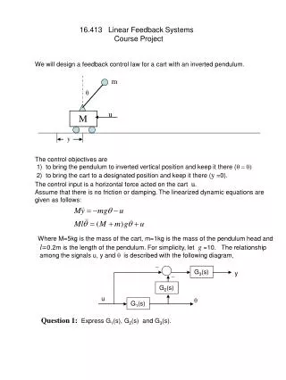
q u M y 16.413 Linear Feedback Systems Course Project We will design a feedback control law for a cart with an inverted pendulum. m The control objectives are 1) to bring the pendulum to inverted vertical position and keep it there (q = 0) 2) to bring the cart to a designated position and keep it there (y=0). The control input is a horizontal force acted on the cart u. Assume that there is no friction or damping. The linearized dynamic equations are given as follows: Where M=5kg is the mass of the cart, m=1kg is the mass of the pendulum head and l=0.2mis the length of the pendulum. For simplicity, let g =10. The relationship among the signals u, y and q is described with the following diagram, - G3(s) y - G2(s) u q G1(s) Question 1: Express G1(s), G2(s) and G3(s).
As+B - G3(s) S - y G2(s) v - q r + + u S Cs+D G1(s) S - The following feedback control strategy is proposed to achieve the control objectives: Since the desired q = 0, r=0. The control strategy correspond to Assume that A and B are already given as A=4, B=1. Question 2: Derive the transfer function from v to q. Question 3: Derive the transfer functions from r to q and from r to y. Question 4: Give conditions for C and D so that the transfer function from r to q is stable. Pick three pairs of (C,D) that satisfy the stability condition. Question 5: Realize the control system with SIMULINK. The initial conditions are Run the system for 20 seconds with each pair of your chosen (C,D). (A recommended sampling period is 0.01 second.) Plot the time responses of u(t), y(t) and q(t) for each case. Question 6: Try your best to explain the difference in transient responses among the three cases. For example, from the location of the closed-loop poles. Question 7: Keep your designed parameters C and D, but set A=B=0. Run the system and see what will happen for the response of q and y. Plot the time responses of u(t), y(t) and q(t) for each of the four cases. Send your Simulink model to me. Demonstrate your results in class. Note: A Matlab code will be provided for you to animate the system with your output signals.