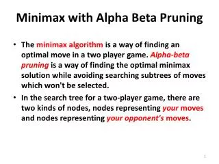
Chapter 8 Performance Analysis of Alpha-Beta Pruning
Chapter 8 Performance Analysis of Alpha-Beta Pruning. Performance analysis of Alpha-Beta Pruning. Since alpha-beta pruning performs a minimax search while pruning much of the tree, its effect is to allow a deeper search with the same amount of computation.

Chapter 8 Performance Analysis of Alpha-Beta Pruning
E N D
Presentation Transcript
Chapter 8 Performance Analysis of Alpha-Beta Pruning
Performance analysis of Alpha-Beta Pruning • Since alpha-beta pruning performs a minimax search while pruning much of the tree, its effect is to allow a deeper search with the same amount of computation. • The question: how much does alpha-beta improve performance? • The best way to characterize is asymptotic effective branching factor. • The dth root of the number of nodes (in a search to depth d, in the limit of large d) • number of nodes generated at depth d / number of nodes generated at depth d-1.
Performance analysis of Alpha-Beta Pruning • The efficiency of alpha-beta pruning depends upon the order in which nodes are encountered at the search frontier. • Thus, we consider 3 different cases: • worst case - the algorithm doesn’t perform any cutoffs at all • best case • average case
MAX MIN 4 4 2 4 8 2 14 4 2 6 8 1 2 12 14 4 5 3 2 6 7 8 9 1 10 2 11 12 13 14 14 Example of alpha-beta worst case • Evaluation from left to right
Lower Bound for Minimax Algorithms • We consider a lower bound on the number of leaf nodes that must be examined by any minimax algorithm. • In minimax algorithm, it’s a guaranty to return the minimax value vof the root node of a game tree. • verifying maximum value = v verifying value v && value v. • Any correct minimax algorithm must explore: • a strategy for Max • a strategy for Min
value v: doesn’t matter what min does Strategy for max: subtree containing: one child of each Max node all b children of each min node value v: doesn’t matter what Max does Strategy for min: subtree containing: one child of each Min node all b children of each Max node Strategies for Min and Max
Example strategy for Min: strategy for Max: Min strategy mixed Max strategy
Strategy for Max d is even leaf nodes d is odd leaf nodes Strategy for Min d is even leaf nodes d is odd leaf nodes Lower Bound for Minimax Algorithms - Analysis • Assume : • uniform branching factor of b uniform depth of d levels • Max move is at the root.
Lower Bound for Minimax Algorithms - Analysis Total number of distinct leaf nodes: • d is odd : • d is even : note: • there is a single leaf node in common of both strategies.
b d/2 + b d/2 -1 = O(bd/2 ) Lower Bound for Minimax Algorithms - Analysis • This is the number of leaf nodes that must be examined by any minimax algorithm. • This is the lower bound of the time complexity.
Minimax value of game trees • The most natural definition for the average case is that the leaf nodes are randomly ordered. • Heuristic node ordering would violate this assumption. • Average case performance is not a prediction of its performance in practice
Minimax value of game trees The root will be in the average case of randomly ordered frontier nodes. • Special case • leaf nodes: • are actual terminal positions, • have the exact values of WIN or LOSS. • Most general case • arbitrary leaf node values
WIN-LOSS Trees analytic model • uniform branching factor b • uniform depth d • Max is to move at the root • depth d is even • terminal nodes labeled WIN with probability P0 • terminal nodes labeled LOSS with probability 1 - P0
Example: Board Splitting • Two players:verticaland horizontal • square sheet of graph paper, bd/2 squares on each side • each square V with probability P0 and H with probability 1 - P0 • vertical’sturn: divides the board vertically into b equals slices, discarding all but one of them.
Board Splitting • horizontal’s turn: divides the board horizontally into b equals slices, discarding all but one of them. • Result: the initial in the only square left indicates the winner.
Pn probability that Max force a win, given that Max is to move 2n moves in the tree Qn probability that Max force a win, given that min is to move 2n -1 moves in the tree Pn Qn Pn-1 Max min Complexity of WIN-LOSS Tree
WIN-LOSS Trees This is the probability that a Max node at any higher level in the tree will be a win for Max
Min is to move to be a win for Max. all of its children must be wins for Max probability that all b children of a node are win for Max Q n = (Pn - 1)b Max is to move to be a loss for Max all of its children must be losses for Max probability that a node is a loss for Max 1 - probability that it is a win for Max 1 - P n = (1 - Q n) WIN-LOSS Trees
WIN-LOSS Trees 1.00 crossover point: determines the probability of a win for Max 0.90 0.80 0.70 0.60 0.50 0.40 0.30 0.20 0.10 0.00 0.00ב 0.20 0.40 0.60 0.80 1.00 Graph showing iterations of function f(x) = 1 - (1 - x2)2.
WIN-LOSS Trees If the probability of a win for MAX at the leaves is grater than crossover point, then the large enough game tree is almost certainly a forced win for MAX!
WIN-LOSS Trees • Let be is the fixed point of the iteration (crossover point). For b = 2, This value is also known as “golden ratio” . • The probability that the root of a game tree is a forced win for Max: Even through wins and losses are chosen randomly at the leaf nodes, we can predict the win-loss status of the root of a sufficiently deep minimax tree with almost certainty, simply by knowing the probability of a win at the leaves!
Minimax convergence theorem • We now generalize our result to the case of leaf nodes with arbitrary numerical values. We adopt a following model: • Uniform branching factor b • uniform depth d • leaves are assigned random numeric value, but from a common probability distribution function Fv0(v) = P(v0 v). • v0 is a particular node value chosen from this distribution
Minimax convergence theorem • Let’s determine the probability distribution of the minimax value of the root of a tree • in the limit of large depth • as a function of the probability distribution of the leaf values • with the expression of the distribution of the minimax values at 2n levels above the leaves as Fvn(v)
Minimax convergence theorem a leaf node is a win for Max its value> v • Minimax value of a max node will be greater than v any one of its children has a minimax value greater than v. For any value of v: • The minimax values propagate up the same as in the win-loss trees. a leaf node is a win for Min its value >v • Minimax value of a min node will be greater than v all of its children has a minimax value greater than v.
The theorem: Minimax convergence theorem • In win-loss treePn is the probability that a Max node 2n levels above the leaves is a forced win for Max. • In general game tree
Minimax convergence theorem The Meaning: • Probability distribution is zero up to a particular value of v (v*). in a b-ary tree: • beyond v*, the probability distribution function of the minimax value of the root is 1. • The probability density function of the step distribution function Fvn(v) is an impulse at v*. All the probability mass is concentrated at v *.
Conclusion for a minimax tree We can predict exactly what the minimax value of the root of the tree will be. • Given: • arbitrary terminal values chosen independently from the same distribution • limit of large depth
Example (application) Goal: • a fuse that will burn out after a specific time. problem: • we only have fuses that have same broad distribution of burn-out time. solution: • we connect two fuses in parallel • the burn-out time of the whole circuit will be the maximum of the burn-out time of the individual fuses • the circuit will remain closed until both fused burn-out • The burn-out time of the entire circuit is the minimax value of the burn-out times of the individuals fuses.
Average-case time complexity - Win-Loss game tree • We assume the previous model. • Assume that According to the minimax convergence theorem, at sufficiently high levels of the tree, all nodes are losses for Max and wins for Min. Max node all the children must be examined all the children will be a loss for Max Min node only the first node must be examined it will be a win for Max
Average-case time complexity - Win-Loss game tree If we follow any path from root, we will branch: • only one way at the alternating Max levels • b ways at every other level @ effective branching factor of b1/2 The asymptotic number of leaf nodes in the limit of large depthO(bd/2 )
Average-case time complexity - Win-Loss game tree • Assume that In this case, at sufficiently high levels of the tree, all nodes are losses for Max and wins for Min. • As the above case, this alse results in effective b.f of b1/2 • Assume that (extremely rare case) • Pearl shows : effective branching factor =
Average-case time complexity - Trees with arbitrary terminal values • There are two possibilities for choosing the leaf values: • a continuous distribution - segment of the real number number line. • Minimax values of all nodes will be equal • Alpha-beta pruning will realize its best performance • a discrete distribution - only a finite number of distinct values. • The probability that any node takes an any particular value is zero • Pearl shows: effective branching factor =
Chapter 9 Multi player games
Introduction • We generalize the 2-player-perfect-information algorithms, to the case of non-cooperative perfect-information -more players games. • No coalitions between players. • Examples: • Chinese Checkers with 6 players. • Othello extended by having different colored pieces for each player.
Maxn (maxn) Algorithm Assumption: • the players alternate moves • each player tries to maximize his/her return • and indifferent to returns of others.
Maxn Algorithm • At frontier nodes, evaluation function returns an n-tuple of values: (player1, P2, P3, …. Player n) • For example: • Othello - return number of pieces for each player.
Maxn Algorithm the entire n-tuple of the child for which the ith component is maximum. evaluation function in each interior node where player i is to move =
(7,3,6) 1 (1,7,2) (7,3,6) 2 2 (6,5,4) (1,7,2) (7,3,6) 3 3 3 3 (3,1,8) (2,8,1) (3,1,8) (1,7,2) (5,6,3) (6,5,4) (8,5,4) (7,3,6) (4,2,7) Maxn Algorithm - Example
Maxn Algorithm • Formal notations: • M(x) - static heuristic value of node x • M(x,p) - backed-up maxn value of node x by player p. • Mi(x,p) - component of M(x,p) corresponds to the return for player i. • M(xi,p’) = maxMp(xi,p’) over children of node x, • p’ is player that follows player p • tie breaking in favor of leftmost node. • Recursive definition of the maxn node:
Maxn Algorithm • Minimax can be viewed as a special case of maxn, when • n = 2, • evaluation function: (x, -x). • Luckhardt & Irani observed: • at nodes where player i is to move, only the ith component of the children need be evaluated. • It may be no less expensive to compute all components. • Without assumptions on values of components, pruning of branches is impossible (with more than 2 players).
Alpha-Beta in multi-Player Games • Tree pruning is possible when : • there is an upper bound on the sum of all components of a tuple • a lower bound on the values of each component. • For example: • Othello - no player can have less than zero, and total number of pieces on the board is equal for all nodes at same level.
Immediate Pruning • Player I is to move, and in one child the ith component equals the upper bound of sum on all components. • Obvious that any other child can be pruned. • This is equivalent to situations in the two-player case when a child of a Max node has value of , or a child of a Min node has value of -, indication a won position for the corresponding player.
(3,3,3) (3, 6, 6) 1 (3,3,3) 2 (2, 7, 2) (3, 6, 3) 2 2 3 3 3 3 3 (3,3,3) (1,6,2) (4,2,3) (3,1,5) (1,7,1) Shallow Pruning
Shallow algorithm Shallow(Node, Player, Bound) IF Node is terminal, RETURN static value Best = Shallow(first Child, next Player, Sum) FOR each remaining Child IF Best[Player] >= Bound, RETURN Best Current = Shallow(Child, next Player, Sum - Best[Player] ) IF Current[Player] > Best[Player], Best = Current RETURN Best
Failure of deep pruning • In a 2-player game, alpha-beta allows deep pruning - pruning a node based on bounds inherited from its great-grandparents, or other distant ancestor. Deep pruning does not generalize to more than 2 players!
(5, 5, 4) 1 2 2 (5,2,2) (4, 4, 5) 3 3 (6,1,2) 1 1 (2,2,5) (2,3,4) or (3,0,6) Failure of Deep Pruning -Example
Optimality of shallow pruning • Theorem: • Every directional algorithm that computes the maxn value of a game tree with more than 2 players must evaluate every terminal node evaluated by shallow pruning under the same order. • Steps of proof: • The formal proof is by induction on the height of the tree and generalizes the result to an arbitrary number of players greater than 2.
Optimality of shallow pruning • Try to see a “zipper” effect in the sense that the original order of the “teeth” (nodes) at the bottom determines the order of the teeth at the top, even though no individual tooth can move very far.
Chapter 10 Minimax and Pathology
Minimax and Pathology • So far, we have considered the time and spacre complexities of minimax search. • We now turn our attention to the quality of the decisions it makes. • Since alpha-beta makes exactly the same decisions as minimax search, the question is the decision quality of minimax.