Image Segmentation Using Physical Models
Image Segmentation Using Physical Models. Yuliya Kopylova CS 867 Computer Vision. Motivation. Motivation for this presentation Provide a few examples where physics models proved to be successful solving open problems in computer vision Walk you through “the mapping process”

Image Segmentation Using Physical Models
E N D
Presentation Transcript
Image SegmentationUsing Physical Models Yuliya Kopylova CS 867 Computer Vision
Motivation • Motivation for this presentation • Provide a few examples where physics models proved to be successful solving open problems in computer vision • Walk you through “the mapping process” • Motivation for this research project • Come up to some new twists to a well-defined problem in physics and see if it can be redefined in the new context
Roadmap • Four examples • Introduction of a phenomenon • Physics behind it • Mapping / analogy • My work • Future work • Conclusion
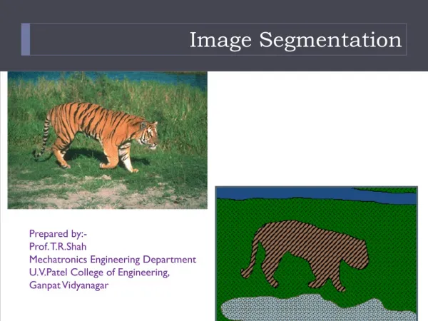
Segmentation Segmentation can be defined as extracting meaningful features from an input image and dividing the image into separate regions based on discontinuities in the feature space. In other words, we want to find a boundary that divides an image into a set of disjoint regions where each region corresponds to a physically meaningful area.
Example 1: Weak Membrane • Imagine an elastic membrane, which we want to fit to a surface • The edges will appear as tears on the membrane • The membrane is described as an elastic energy function of a membrane that can be minimized to achieve equilibrium
Example 2: Dipole Field • Imagine magnetic dipoles interacting with each other. Treat edges as dipoles • Each dipole affects the orientation and the strength of diploes in immediate neighborhood • Edge fragments can be connected by tracings the EM field vector • A configuration with a smaller energy represents a perceptually pleasing edge configuration
Example3: Granular Ferromagnet • Each point has a magnetic moment (spin) • Ferromagnetic interaction is introduced between each pair of neighboring spins • At temperature T=0 spins are all aligned • At high temperatures the system is totally disordered • As T decreases, the single ferromagnet will break into several grains
Example3: Granular Ferromagnet • Clusters are analogous to ordered regions of spin • Place spin variable at each point • Introduce ferromagnetic interaction between pairs of neighboring spins • Define neighbors as points sharing the same boundary • Remove/freeze bonds between neighbors with probability P
Example 4: Viscous Fluid Model • Imagine particle interaction in highly viscous liquid (to avoid oscillation) • Place N particles on N-1 dimensional sphere • Each particle will interact with its neighbors
Example 4: Viscous Fluid Model • To avoid collapse towards the origin or a run-away to infinity • To ensure fairness of the original placement of the particles (symmetric and completely unbiased) • To simplify calculations of the initial placement
Example 4: Viscous Fluid Model • Calculate gradient which will be equivalent to the forces in action • Place pixels on n-1 dimensional sphere(have to keep track of their coordinates) • Increment time and calculate distances • Continue until no changes observed
Pros Well defined Solution exists gratification Cons Non trivial mapping Complicated Background Assumptions Local minima Can be misleading Conclusion

