Download
1 / 20
200 likes | 215 Vues
Explore how to pack vectors into fewer dimensions while preserving distances for quicker cosine computation. Learn about Latent Semantic Indexing and Random Projection methods, dimensionality reduction, Singular Value Decomposition, and more linear algebra techniques. Discover the concept of Random Projections and the Johnson-Linderstrauss Lemma, providing insights into efficient computation and data reduction. Understand the trade-offs between various techniques for optimal efficiency.

E N D
Packing to fewer dimensions Paolo Ferragina Dipartimento di Informatica Università di Pisa
Speeding up cosine computation • What if we could take our vectors and “pack” them into fewer dimensions (say 50,000100) while preserving distances? • Now, O(nm) to compute cos(d,q) for all n docs • Then, O(km+kn) where k << n,m • Two methods: • “Latent semantic indexing” • Random projection
Briefly • LSI is data-dependent • Create a k-dim subspace by eliminating redundant axes • Pull together “related” axes – hopefully • car and automobile • Random projection is data-independent • Choose a k-dim subspace that guarantees good stretching properties with high probability between any pair of points. What about polysemy ?
Sec. 18.4 Latent Semantic Indexing courtesy of Susan Dumais
Example Notions from linear algebra • Matrix A, vector v • Matrix transpose (At) • Matrix product • Rank • Eigenvalues l and eigenvector v: Av = lv
Overview of LSI • Pre-process docs using a technique from linear algebra called Singular Value Decomposition • Create a new (smaller) vector space • Queries handled (faster) in this new space
Singular-Value Decomposition • Recall mn matrix of terms docs, A. • A has rank r m,n • Define term-term correlation matrix T=AAt • T is a square, symmetric mm matrix • Let U be mrmatrix of r eigenvectors of T • Define doc-doc correlation matrix D=AtA • D is a square, symmetric nn matrix • Let V be nrmatrix of r eigenvectors of D
A’s decomposition • Given U(for T, mr) and V(for D, nr) formed by orthonormal columns (unit dot-product) • It turns out that A = U SVt • WhereS is a diagonal matrix with the eigenvalues of T=AAt in decreasing order. mn mr rn = rr Vt S U A
document k k 0 k 0 0 useless due to 0-col/0-row of Sk Dimensionality reduction • Fix some k << r, zeroout all but the k biggest eigenvalues in S[choice of k is crucial] • Denote by Sk this new version of S, having rank k • Typically k is about 100, while r (A’s rank) is > 10,000 = r Vt S Sk A U Ak k x n r x n m x r m x k
Guarantee • Akis a pretty good approximation to A: • Relative distances are (approximately) preserved • Of all mn matrices of rank k, Ak is the best approximation to A wrt the following measures: • minB, rank(B)=k ||A-B||2 = ||A-Ak||2 = sk+1 • minB, rank(B)=k ||A-B||F2 = ||A-Ak||F2 = sk+12+ sk+22+...+ sr2 • Frobenius norm ||A||F2 = s12+ s22+...+ sr2
U,V are formed by orthonormal eigenvectors of the matrices D,T Reduction • Since we are interested in doc/doc correlation, we consider: • D=AtA=(U SV t)t(U SV t) = (SV t)t (SV t) • Hence X = S Vt is a matrix r x n, may play the role of A • To reduce its size we set Xk = Sk Vt is a matrix k x nand thus get AtA Xkt Xk (both are n x n matrices) • We use Xkto define how to project A: • Since Xk= SkVkt Xk= Ukt A (use def of SVD of A) • Since Xkmay play role of A, its cols are proj. docs • Similarly Q can be interpreted as a new col of A and thus it is enough to multiply Ukt times Q to get the projected query, O(km) time
Which are the concepts ? • c-th concept = c-th col of Uk(which is m x k) • Uk[i][c] = strength of association between c-th concept and i-th term • Vtk[c][j] = strength of association between c-th concept and j-th document • Projected document: d’j=Utkdj • d’j [c] = strenght of concept c in dj • Projected query: q’= Utkq • q’[c] = strenght of concept c in q
Random Projections Paolo Ferragina Dipartimento di Informatica Università di Pisa Slides only !
An interesting math result Lemma (Johnson-Linderstrauss, ‘82) Let P be a set of n distinct points in m-dimensions. Given e > 0, there exists a function f : P IRk such that for every pair of points u,v in P it holds: (1 - e) ||u - v||2 ≤ ||f(u) – f(v)||2 ≤(1 + e) ||u-v||2 Where k = O(e-2 log n) f() is called JL-embedding Setting v=0 we also get a bound on f(u)’s stretching!!!
What about the cosine-distance ? f(u)’s, f(v)’s stretching substituting formula above for ||u-v||2
E[pi,j] = 0 Var[pi,j] = 1 How to compute a JL-embedding? If we set the projection matrix P = pi,j as a random m x k matrix, where its components are independent random variables with one of the following two distributions: 2
Finally... • Random projections hide large constants • k (1/e)2 * log n, so k may be large… • it is simple and fast to compute • LSI is intuitive and may scale to any k • optimal under various metrics • but costly to compute, do exist good libraries