Perceptron Learning Algorithm - Neural Networks Lecture 6
This lecture discusses the Perceptron Learning Algorithm, including the steps involved in training a perceptron and how it can be visualized using linear algebra concepts. It also explores the limitations and potential for generalization of the algorithm.

Perceptron Learning Algorithm - Neural Networks Lecture 6
E N D
Presentation Transcript
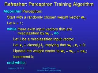
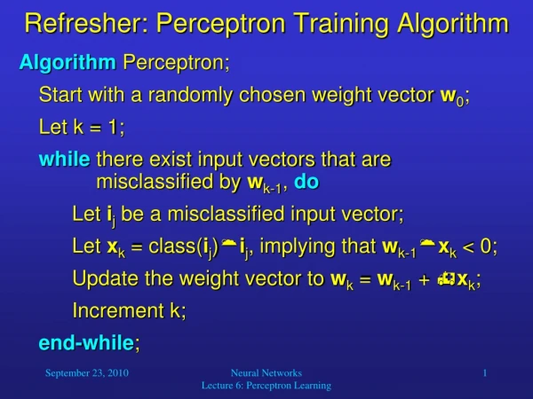
Refresher: Perceptron Training Algorithm • AlgorithmPerceptron; • Start with a randomly chosen weight vector w0; • Let k = 1; • while there exist input vectors that are misclassified by wk-1, do • Let ij be a misclassified input vector; • Let xk = class(ij)ij, implying that wk-1xk < 0; • Update the weight vector to wk = wk-1 + xk; • Increment k; • end-while; Neural Networks Lecture 6: Perceptron Learning
Another Refresher: Linear Algebra • How can we visualize a straight line defined by an equation such as w0 + w1i1 + w2i2 = 0? • One possibility is to determine the points where the line crosses the coordinate axes: • i1 = 0 w0 + w2i2 = 0 w2i2 = -w0 i2 = -w0/w2 • i2 = 0 w0 + w1i1 = 0 w1i1 = -w0 i1 = -w0/w1 • Thus, the line crosses at (0, -w0/w2)T and (-w0/w1, 0)T. • If w1 or w2 is 0, it just means that the line is horizontal or vertical, respectively. • If w0 is 0, the line hits the origin, and its slope i2/ii is:w1i1 + w2i2 = 0 w2i2 = -w1i1 i2/i1 = -w1/w2 Neural Networks Lecture 6: Perceptron Learning
3 i2 2 1 -3 -2 -1 1 2 3 i1 -1 -2 -3 Perceptron Learning Example We would like our perceptron to correctly classify the five 2-dimensional data points below. Let the random initial weight vector w0 = (2, 1, -2)T. Then the dividing line crosses at (0, 1)T and (-2, 0)T. -1 Let us pick the misclassified point (-2, -1)T for learning: i = (1, -2, -1)T (include offset 1) x1 = (-1)(1, -2, -1)T (i is in class -1) x1= (-1, 2, 1)T 1 class -1 class 1 Neural Networks Lecture 6: Perceptron Learning
3 i2 2 1 -3 -2 -1 1 2 3 i1 -1 -2 -3 Perceptron Learning Example w1 = w0 + x1 (let us set = 1 for simplicity) w1= (2, 1, -2)T + (-1, 2, 1)T = (1, 3, -1)T The new dividing line crosses at (0, 1)T and (-1/3, 0)T. Let us pick the next misclassified point (0, 2)T for learning: i = (1, 0, 2)T (include offset 1) x2 = (1, 0, 2)T (i is in class 1) -1 1 class -1 class 1 Neural Networks Lecture 6: Perceptron Learning
3 i2 2 1 -3 -2 -1 1 2 3 i1 -1 -2 -3 Perceptron Learning Example w2 = w1 + x2 w2 = (1, 3, -1)T + (1, 0, 2)T = (2, 3, 1)T Now the line crosses at (0, -2)T and (-2/3, 0)T. With this weight vector, the perceptron achieves perfect classification! The learning process terminates. In most cases, many more iterations are necessary than in this example. 1 -1 class -1 class 1 Neural Networks Lecture 6: Perceptron Learning
Perceptron Learning Results • We proved that the perceptron learning algorithm is guaranteed to find a solution to a classification problem if it is linearly separable. • But are those solutions optimal? • One of the reasons why we are interested in neural networks is that they are able to generalize, i.e., give plausible output for new (untrained) inputs. • How well does a perceptron deal with new inputs? Neural Networks Lecture 6: Perceptron Learning
Perceptron Learning Results Perfect classification of training samples, but may not generalize well to new (untrained) samples. Neural Networks Lecture 6: Perceptron Learning
Perceptron Learning Results This function is likely to perform better classification on new samples. Neural Networks Lecture 6: Perceptron Learning
Adalines • Idea behind adaptive linear elements (Adalines): • Compute a continuous, differentiable error function between net input and desired output (before applying threshold function). • For example, compute the mean squared error (MSE) between every training vector and its class (1 or -1). • Then find those weights for which the error is minimal. • With a differential error function, we can use the gradient descent technique to find this absolute minimum in the error function. Neural Networks Lecture 6: Perceptron Learning
Gradient Descent • Gradient descent is a very common technique to find the absolute minimum of a function. • It is especially useful for high-dimensional functions. • We will use it to iteratively minimizes the network’s (or neuron’s) error by finding the gradient of the error surface in weight-space and adjusting the weights in the opposite direction. Neural Networks Lecture 6: Perceptron Learning
f(x) slope: f’(x0) x0 x1 = x0 - f’(x0) x Gradient Descent • Gradient-descent example: Finding the absolute minimum of a one-dimensional error function f(x): Repeat this iteratively until for some xi, f’(xi) is sufficiently close to 0. Neural Networks Lecture 6: Perceptron Learning
Gradient Descent • Gradients of two-dimensional functions: The two-dimensional function in the left diagram is represented by contour lines in the right diagram, where arrows indicate the gradient of the function at different locations. Obviously, the gradient is always pointing in the direction of the steepest increase of the function. In order to find the function’s minimum, we should always move against the gradient. Neural Networks Lecture 6: Perceptron Learning