Download
1 / 19
190 likes | 207 Vues
Explore the dynamics of convergent plate margins, from subduction zones to seismic energy release, paired metamorphic belts, and the anatomy of subduction complexes. Learn about the forces at play, phase transitions, and seismicity in these complex geological regions.

E N D
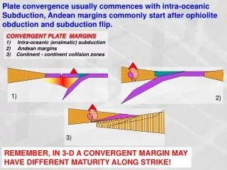
Plate convergence usually commences with intra-oceanic Subduction, Andean margins commonly start after ophiolite obduction and subduction flip. CONVERGENT PLATE MARGINS Intra-oceanic (ensimatic) subduction Andean margins 3) Continent - continent collision zones 1) 2) 3) REMEMBER, IN 3-D A CONVERGENT MARGIN MAY HAVE DIFFERENT MATURITY ALONG STRIKE!
legend and estimates of forces • Fsp - Slab-pull(+) • Frp - Ridge-push(+) • Fsu - Suctional force (+) • For - Orogenic spreading(+) • Fdf - Mantle drag-force (+ or -) • Fsr - Subduction ressistance (-) • Fcd - Extra continental-drag(-) • Ftr - Transform resistance (-) Frp = ge(m – w) (L/3 +e/2) ≈ 2*1012 Nm-1 g - gravity ≈ 9,8 ms-2 e – elevation of spreading ridge above cold plate ≈ 3,3 km m – mantle density, ≈ 3,3 g cm-3w – water density L – lithosphere thickness ≈ 85km
Estimate of slab-pull force Fsp pr. unit length subduction zone (see Fowler: Solid Earth, Chap 7, for details) 2z 8gm T1L2Re 2d Fsp(z) = [exp(- ) - exp(- )] = ca 2*1013Nm-1 4 2ReL 2ReL • z – depth (d = z give Fsp = 0) • – coeficient of thermal expansion • T1 – mantle temp, • d+L – thickness of the upper mantle • L – Lithosphere (plate) thickness • Re – Thermal Reynolds number Re =(mcpvL)/2k Thermal Reynolds number k - conductivity cp - spesific heat k - kinematic viscosity v - subd. velocity
Reactions and phase transitions affecting the forces in subduction zones • In addition to the thermal contraction and density change will the forces of the subducting litosphere be affected by • Gabbro to eclogite transition (+) • Olivin-spinel transiton (+) • Spinel to oxides (perovskitt and periklas) (-)
Modeled density structure of subducted MORB, Hacker et al. 2003
Temperature variation across a subduction zone • Notice the localization of the olivin-spinel and spinel-oxide transitions. • Use the next fig to explain the phenomena
Phase diagrams for the transititions for olivin to spinel and spinel to post-spinel (oxides)
THE ANATOMY OF A SUBDUCTION COMPLEX Outer non-volcanic island Fore-arc basin Active volcanic arc Remnant-arcs from arc-splitting Back-arc basin/spreading alternating compression amd tension Compression Tension Trench sea level High geotherm Low geotherm Accreationary prism High geotherm Please notice that Benioff zones frequently have an irregular shape in 3-D (ex. Banda Arc). 80% of all seismic energy is released in Benioff zones. The low geotherm in subductions zones makes them the prime example of high P - low T regional metamorphic complexes. The high geotherm in the arc-region gives contemporaneous high-T low P regional metamorphism, together these two regions give rise to a feature known as”Paired Metamorphic Belts”
Accreationary Prism, Example from Scotland. Age: Late Ordovician to Late Silurian ca 450-420 Ma
Blueshists normally originate here! Ophiolites normally originate here! alternating compression amd tension Compression Tension Trench sea level High geotherm Low geotherm High geotherm Seismic quality factor (Q): The ability to transmitt seismic energy without loosing the energy. Low Q in high-T regions. Seismic quiet zones---NB potential build-up to very large quakes! Arc-splitting - tensional regime above subductions zones. Subduction roll-back. High heat-flow in the supra-subductions zone regime give rise to relatively low shallow sealevel above the back-arc basins. Most ophiolite complexes have their origin is a supra-subduction environment
3 - D MORPHOLOGY NB! NOTICE INTRA-SLAB EARTHQUAKES SEISMICITY
Link: fault plane solution Link: displacement magnitude Link: earthquake information in general
The amount of energy radiated by an earthquake is a measure of the potential for damage to man-made structures. Theoretically, its computation requires summing the energy flux over a broad suite of frequencies generated by an earthquake as it ruptures a fault. Because of instrumental limitations, most estimates of energy have historically relied on the empirical relationship developed by Beno Gutenberg and Charles Richter: log10E = 11.8 + 1.5MS where energy, E, is expressed in ergs. The drawback of this method is that MS is computed from an bandwidth between approximately 18 to 22s. It is now known that the energy radiated by an earthquake is concentrated over a different bandwidth and at higher frequencies. With the worldwide deployment of modern digitally recording seismograph with broad bandwidth response, computerized methods are now able to make accurate and explicit estimates of energy on a routine basis for all major earthquakes. A magnitude based on energy radiated by an earthquake, Me, can now be defined, Me = 2/3 log10E - 2.9. For every increase in magnitude by 1 unit, the associated seismic energy increases by about 32 times. Although Mw and Me are both magnitudes, they describe different physical properites of the earthquake. Mw, computed from low-frequency seismic data, is a measure of the area ruptured by an earthquake. Me, computed from high frequency seismic data, is a measure of seismic potential for damage. Consequently, Mw[MW = 2/3 log10(MO) - 10.7] and Me often do not have the same numerical value.
Frictional heating on faults may result in melting of any rock-coposition
Stress-measurements from grain-size and dislocation density (4 to 5 x10¹³m-2) in olivine associated with pseudotachylytes in peridotite indicate that peridotites (mantle rocks) may sustain extreme differential stress: 1-3≈ 3-600 MPa. Assuming a fault with a modest displacement of d ≈ 1m, and a differential stress of 300 MPa the release of energy according to equation (1): Wf = Q + E where Q = heat and E = seismic energy is Wf = d n = d (1-3)/2 =1m(300MPa)/2 ≈ 1.5 x 10⁸ J m-2 or 47 kWhm-2. The seismic energy (E) is commonly estimated to be < 5% of Wf on a strong fault, ie. less than 2.3 kWh m-2 is radiated as seismic waves, the remaining energy (Q) turns to heat and surface energy (difficult to measure) along the fault. The process is adiabatic since the fault movement occurs in seconds and no heat is lost by conduction (thermal diffusivity ~1.5 mm2s-1). Taking the heat capacity of lherzolite, Cp = 1150 J kg-1 oC-1 and a heat of fusion (Fo) H = 8.6 x10⁶ Jkg-1 the thermal energy (equation 4) required to melt one kg of peridotite: (4) Q = Cp(T) + H = 1150Jkg-1oC-1 (1200oC) + 8.6 x10⁶ Jkg-1 = 2.7 x 10⁵ Jkg-1. On a fault with D = 1m, ~60 kg lherzolite may melt pr m2 of the fault plane, corresponding to an approximately 2 cm thick layer of ultramafic pseudotachylyte.