Overview of Speech Recognition using Dynamic Time Warping (DTW)
Learn about historical background, mathematical concepts, feature extraction, audio signal processing, template matching, time normalization, DTW complexity, DTW-based techniques, and endpoint detection in Automatic Speech Recognition (ASR) systems.

Overview of Speech Recognition using Dynamic Time Warping (DTW)
E N D
Presentation Transcript
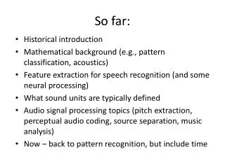
So far: • Historical introduction • Mathematical background (e.g., pattern classification, acoustics) • Feature extraction for speech recognition (and some neural processing) • What sound units are typically defined • Audio signal processing topics (pitch extraction, perceptual audio coding, source separation, music analysis) • Now – back to pattern recognition, but include time
Sequence recognition for ASR • ASR = static pattern classification + sequence recognition • Deterministic sequence recognition: template matching • Templates are typically word-based;don’t need phonetic sound units per se • Still need to put together local distances into something global (per word or utterance)
Front end analysis • Basic approach the same for deterministic, statistical: • 25 ms windows (e.g., Hamming), 10 ms steps (a frame) • Some kind of cepstral analysis (e.g., MFCC or PLP) • Cepstral vector at time n called xn
Speech sound categories • Words, phones most common • For template-based ASR, mostly words • For template-based ASR, local distances based on examples (reference frames) versus input frames
From Frames to Sequence • Easy if local matches are all correct (never happens!) • Local matches are unreliable • Need measure of goodness of fit • Need to integrate into global measure • Need to consider all possible sequences
Templates: Isolated Word Example • Matrix for comparison between frames • Word template = multiple feature vectors • Reference template = • Input template = • Need to find D( , )
Templates Matching Problem • Time Normalization • Which references to use • Defining distances/costs • Endpoints for input templates
Time Normalization • Linear Time Normalization • Nonlinear Time Normalization – Dynamic Time Warp (DTW)
Linear Time Normalization: Limitations • Speech sounds stretch/compress differently • Stop consonants versus vowels • Need to normalize differently
Generalized Time Warping • Permit many more variations • Ideally, compare all possible time warpings • Vintsyuk (1968): use dynamic programming
Dynamic programming • Bellman optimality principle (1962): optimal policy given optimal policies from sub problems • Best path through grid: if best path goes through grid point, best path includes best partial path to grid point • Classic example: knapsack problem
Knapsack problem • Stuffing a sack with items, different value • Goal: maximize value in sack • Key point 1: If max size is 10, and we know values of solutions for max size of 9, we can compute the final answer knowing the value of adding items. • Key point 2: Point 1 sounds recursive, but can be made efficiently nonrecursive by building a table
Basic DTW step w/ simple local constraints. Each (i,j) cell has local distance d and cumulative distortion D. The eqn shows the basic computational step.
Dynamic Time Warp (DTW) • Apply DP to ASR: Vintsyuk, Bridle, Sakoe • Let D(i,j) = total distortion up to frame i in input and frame j in reference • Let d(i,j) = local distance between frame i in input and frame j in reference • Let p(i,j) = set of possible predecessors toframe i in input and frame j in reference • D(i,j) = d(i, j) + minp(i,j) D(p(i,j))
DTW steps (1) Compute local distance d in 1st column(1st frame of input) for each reference template.Let D(0,j) = d(0,j) for each cell in each template (2) For i=1 (2nd column), j=0, compute d(i,j) add to min of all possible predecessor values of D to get local value of D; repeat for each frame in each template. (3) Repeat (2) for each column to the end of input (4) For each template, find best D in last column of input (5) Choose the word for the template with smallest D
DTW Complexity • O(Nframesref. Nframesin . Ntemplates) • Storage, though can just be O(Nframesref. Ntemplates) (store current column and previous column) • Constant reduction: global constraints • Constant reduction: local constraints
Which reference templates? • All examples? • Prototypes? • DTW-based global distances permit clustering
DTW-based K-means • (1) Initialize (how many, where) • (2) Assign examples to closest center (DTW distance) • (3) For each cluster, find template with minimum value for maximum distance, call it the center • (4) Repeat (2) and (3) until some stopping criterion is reached • (5) Use center templates as references for ASR
Defining local distance • Normalizing for scale • Cepstral weighting • Perceptual weighting, e.g., JND • Learning distances, e.g., with ANN, statistics
Endpoint detection: big problem! • Sounds easy • Hard in practice (noise, reverb, gain issues) • Simple systems use energy, time thresholds • More complex ones also use spectrum • Can be tuned • Not robust
Connected Word ASR by DTW • Time normalization • Recognition • Segmentation • Can’t have templates for all utterances • DP to the rescue
DP for Connected Word ASR by DTW • Vintsyuk, Bridle, Sakoe • Sakoe: 2-level algorithm • Vintsyuk, Bridle: one stage • Ney explanationNey, H., “The use of a one-stage dynamic programming algorithm for connected word recognition,” IEEE Trans. Acoust. Speech Signal Process. 32: 263-271, 1984
Connected Algorithm • In principle: one big distortion matrix(for 20,000 words, 50 frames/word, 1000 frame input [10 seconds] would be 109 cells!) • Also required, backtracking matrix (since word segmentation not known) • Get best distortion • Backtrack to get words • Fundamental principle: find best segmentation and classification as part of the same process, not as sequential steps
DTW for connected words • In principle, backtracking matrix points backto best previous cell • Mostly just need backtrack to end of previous word • Simplifications possible
Storage efficiency • Distortion matrix -> 2 columns • Backtracking matrix -> 2 rows • “From template” points to template with lowest cost ending here • “From frame” points to end frame of previous word
More on connected templates • “Within word” local constraints • “Between word” local constraints • Grammars • Transition costs
Knowledge-based segmentation • DTW combines segmentation, time norm, recognition; all segmentations considered • Same feature vectors used everywhere • Could segment separately, using acoustic-phonetic features cleverly • Example: FEATURE, Ron Cole (1983)
Limitations of DTW approach • No structure from subword units • Average or exemplar values only • Cross-word pronunciation effects not handled • Limited flexibility for distance/distortion • Limited mathematical basis • -> Statistics!
Epilog: “episodic” ASR • Having examples can get interesting again when there are many of them • Potentially an augmentation of stat methods • Recent experiments show decent results • Somewhat different properties -> combination
The rest of the course • Statistical ASR • Speech synthesis • Speaker recognition • Speaker diarization • Oral presentations on your projects • Written report on your project
Class project timing • Week of April 30: no class Monday, double class Wednesday May 2 (is that what people want?) • 8 oral presentations by individuals, 12 minutes each + 3 minutes for questions • 2 oral presentations by pairs – 17 minutes each + 3 minutes for questions • 3:10 PM to 6 PM with a 10 minute mid-session break • Written report due Wednesday May 9, no late submissions (email attachment is fine)