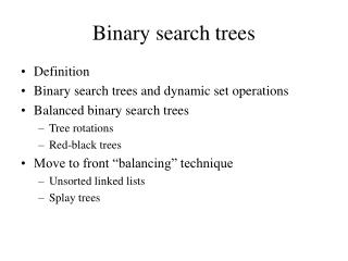
Binary Search Trees: Lecture Notes and Applications
This lecture covers the concept of binary search trees, including insertion and deletion operations, querying on dynamic sets, edge paths, node properties, and various applications such as expression and game trees.

Binary Search Trees: Lecture Notes and Applications
E N D
Presentation Transcript
Lecture 11:Binary Search Trees Shang-Hua Teng
Keys Keys Entry Satellite data Data Format
Insertion and Deletion on dynamic sets • Insert(S,x) • A modifying operation that augments the set S with the element pointed by x • Delete • Given a pointer x to an element in the set S, removes x from S • Notice that this operation uses a pointer to an element x, not a key value
Querying on dynamic sets • Search(S,k) • given a set S and a key value k, returns a pointer x to an element in S such that key[x] = k, or NIL if no such element belongs S • Minimum(S) • on a totally ordered set S that returns a pointer to the element S with the smallest key • Maximum(S) • Successor(S,x) • Given an element x whose key is from a totally ordered set S, returns a pointer to the next larger element in S, or NIL if x is the maximum element • Predecessor(S,x)
Edge interior node path Node subtree leaf child Trees root Degree? parent Depth/Level? Height?
Parent Data Left Right root • Tree • root Binary Tree • Node • data • left child • right child • parent (optional)
Trees • Full tree of height h • all leaves present at level h • all interior nodes full • total number of nodes in a full binary tree? • Complete tree of height h
+ * - 5 3 8 4 Applications - Expression Trees To represent infix expressions (5*3)+(8-4)
Applications - Parse Trees Used in compilers to check syntax statement statement else statement if cond then statement if cond then
Binary Search Trees • Binary Search Trees (BSTs) are an important data structure for dynamic sets • In addition to satellite data, elements have: • key: an identifying field inducing a total ordering • left: pointer to a left child (may be NULL) • right: pointer to a right child (may be NULL) • p: pointer to a parent node (NULL for root)
F B H A D K Binary Search Trees • BST property: key[leftSubtree(x)] key[x] key[rightSubtree(x)] • Example:
Pre order visit the node go left go right In order go left visit the node go right Post order go left go right visit the node Level order / breadth first for d = 0 to height visit nodes at level d Traversals for a Binary Tree
A B C D E F G H I Traversal Examples Pre order A B D G H C E F I In order G D H B A E C F I Post order G H D B E I F C A Level order A B C D E F G H I
Traversal Implementation • recursive implementation of preorder • base case? • self reference • visit node • pre-order(left child) • pre-order(right child) • What changes need to be made for in-order, post-order?
Inorder Tree Walk • In order TreeWalk(x) TreeWalk(left[x]); print(x); TreeWalk(right[x]); • Prints elements in sorted (increasing) order
F B H A D K In order Tree Walk • Example: • How long will a tree walk take? • In order walk prints in monotonically increasing order. Why?
+ * - 5 3 8 4 Evaluating an expression tree • Walk the tree in postorder • When visiting a node, use the results of its children to evaluate it.
Operations on BSTs: Search • Given a key and a pointer to a node, returns an element with that key or NULL: TreeSearch(x, k) if (x = NULL or k = key[x]) return x; if (k < key[x]) return TreeSearch(left[x], k); else return TreeSearch(right[x], k);
F B H A D K BST Search: Example • Search for D and C:
Operations of BSTs: Insert • Adds an element x to the tree so that the binary search tree property continues to hold • The basic algorithm • Like the search procedure above • Insert x in place of NULL • Use a “trailing pointer” to keep track of where you came from (like inserting into singly linked list)
F B H A D K BST Insert: Example • Example: Insert C C
BST Search/Insert: Running Time • What is the running time of TreeSearch() or TreeInsert()? • O(h), where h = height of tree • What is the height of a binary search tree? • worst case: h = O(n) when tree is just a linear string of left or right children • We’ll keep all analysis in terms of h for now • Later we’ll see how to maintain h = O(lg n)
Animation • Animated Binary Tree
Sorting With Binary Search Trees • Informal code for sorting array A of length n: BSTSort(A) for i=1 to n TreeInsert(A[i]); InorderTreeWalk(root); • Argue that this is (n lg n) • What will be the running time in the • Worst case? • Average case? (hint: remind you of anything?)
3 1 8 2 6 5 7 Sorting With BSTs for i=1 to n TreeInsert(A[i]); InorderTreeWalk(root); • Average case analysis • It’s a form of quicksort! 3 1 8 2 6 7 5 1 2 8 6 7 5 2 6 7 5 5 7
Sorting with BSTs • Same partitions are done as with quicksort, but in a different order • In previous example • Everything was compared to 3 once • Then those items < 3 were compared to 1 once • Etc. • Same comparisons as quicksort, different order!
Sorting with BSTs • Since run time is proportional to the number of comparisons, same expected time as quicksort: O(n lg n) • Which do you think is better, quicksort or BSTsort? Why?
Sorting with BSTs • Since run time is proportional to the number of comparisons, same time as quicksort: O(n lg n) • Which do you think is better, quicksort or BSTSort? Why? • Answer: quicksort • Better constants • Sorts in place • Doesn’t need to build data structure
More BST Operations • A priority queue supports • Insert • Minimum • Extract-Min • BSTs are good for more than sorting. For example, can implement a priority queue
BST Operations: Minimum • How can we implement a Minimum() query? • What is the running time? • O(h)
BST Operations: Successor • For deletion, we will need a Successor() operation • Draw Fig 13.2 • What is the successor of node 3? Node 15? Node 13? • What are the general rules for finding the successor of node x? (hint: two cases)
BST Operations: Successor • Two cases: • x has a right subtree: successor is minimum node in right subtree • x has no right subtree: successor is first ancestor of x whose left child is also ancestor of x • Intuition: As long as you move to the left up the tree, you’re visiting smaller nodes. • Predecessor: similar algorithm
F Example: delete Kor H or B B H C A D K BST Operations: Delete • Deletion is a bit tricky • 3 cases: • x has no children: • Remove x • x has one child: • Splice out x • x has two children: • Swap x with successor • Perform case 1 or 2 to delete it
BST Operations: Delete • Why will case 2 always go to case 0 or case 1? • because when x has 2 children, its successor is the minimum in its right subtree • Could we swap x with predecessor instead of successor? • Of course
Next Lecture • Up next: guaranteeing an O(lg n) height tree
Dictionary/Table Keys Operation supported: search Given a student ID find the record (entry)
Keys Entry Data Format
What if student ID is 9-digit social security number • Well, we can still sort by the ids and apply binary search. • If we have n students, we need O(n) space • And O(log n) search time
What if new students come and current students leave • Dynamic dictionary • Yellow page update once in a while • Which is not truly dynamic • Operations to support • Insert: add a new (key, entry) pair • Delete: remove a (key, entry) pair from the dictionary • Search: Given a key, find if it is in the dictionary, and if it is , return the data record associated with the key
How should we implement a dynamic dictionary? • How often are entries inserted and removed? • How many of the possible key values are likely to be used? • What is the likely pattern of searching for keys?
key entry “Smith” “Smith”, “124 Hawkers Lane”, “9675846” “Yeo” “Yeo”, “1 Apple Crescent”, “0044 1970 622455” (Key,Entry) pair • For searching purposes, it is best to store the key and the entry separately (even though the key’s value may be inside the entry) (key,entry)
Implementation 1:unsorted sequential array • An array in which (key,entry)-pair are stored consecutively in any order • insert: add to back of array; O(1) • search: search through the keys one at a time, potentially all of the keys; O(n) • remove: find + replace removed node with last node; O(n) key entry 0 1 2 3 … and so on
Implementation 2:sorted sequential array • An array in which (key,entry) pair are stored consecutively, sorted by key • insert: add in sorted order; O(n) • find: binary search; O(log n) • remove: find, remove node and shuffle down; O(n) key entry 0 1 2 3 … and so on
Implementation 3:linked list (unsorted or sorted) • (key,entry) pairs are again stored consecutively • insert: add to front; O(1)or O(n) for a sorted list • find: search through potentially all the keys, one at a time; O(n)still O(n) for a sorted list • remove: find, remove using pointer alterations; O(n) key entry and so on
Direct Addressing • Suppose: • The range of keys is 0..m-1 (Universe) • Keys are distinct • The idea: • Set up an array T[0..m-1] in which • T[i] = x if x T and key[x] = i • T[i] = NULL otherwise
0 / entry 1 1 2 / 3 / 7 4 / 1 5 5 5 6 / 7 7 Direct-address Table • Direct addressing is a simple technique that works well when the universe of keys is small. Assuming each key corresponds to a unique slot. Direct-Address-Search(T,k) return T[k] Direct-Address-Insert(T,x) return T[key[x]] x Direct-Address-Delete(T,x) return T[key[x]] Nil O(1) time for all operations
The Problem With Direct Addressing • Direct addressing works well when the range m of keys is relatively small • But what if the keys are 32-bit integers? • Example: spell checking • Problem 1: direct-address table will have 232 entries, more than 4 billion • Problem 2: even if memory is not an issue, the time to initialize the elements to NULL may be • Solution: map keys to smaller range 0..m-1 • This mapping is called a hash function
T 0 U(universe of keys) h(k1) k1 h(k4) k4 K(actualkeys) k5 h(k2) = h(k5) k2 h(k3) k3 m - 1 Hash function • A hash function determines the slot of the hash table where the key is placed. • Previous example the hash function is the identity function • We say that a record with key k hashes into slot h(k)
Next Problem • collision T 0 U(universe of keys) h(k1) k1 h(k4) k4 K(actualkeys) k5 h(k2) = h(k5) k2 h(k3) k3 m - 1