Models with reduced vertical structure
Models with reduced vertical structure. Adam Sobel Banff Summer School. Vertical discretizations, 0: N-level system. Level models are derived by numerical discretization of the equations, by a finite-difference method or something

Models with reduced vertical structure
E N D
Presentation Transcript
Models with reduced vertical structure Adam Sobel Banff Summer School
Vertical discretizations, 0: N-level system Level models are derived by numerical discretization of the equations, by a finite-difference method or something close to it; a mathematical, rather than a physical argument. We can then just choose to use a small number of levels.
Vertical discretizations, 1: N-layer system Consider a stack of N layers of fluid, each of constant density i, and assumed to move with velocity ui, both uniform within each layer. Let the top surface be either free, or rigid. Mean layer thicknesses Hi, displacements i N N, uN The motions of the system can be expressed in terms of the ui, and i. We get a set of shallow-water equations, coupled through the interface displacements (which affect the pressure gradients) … H 3, u3 2, u2 1 1, u1 H1
Vertical discretizations, 2a: Modal decomposition from the layers Alternatively, we can decompose the motion into modes. We label the modes with indeces. The gravest or “barotropic” mode has all ui equal, and has the largest surface displacement (or surface pressure if rigid lid). The next, or “first baroclinic” has the lower half moving in sync, out of phase with the upper half. The higher order modes have increasingly finer vertical structure. Let the amplitude of each velocity mode be Uj(x,t).
Vertical discretizations, 2b: Modal decomposition from the layers The modes are complete; we can reconstruct the layer motions with ui=j uij Uj(x,t). The uij are the vertical structures; they tell us how much layer i moves per unit amplitude of mode j. Under linear dynamics, the modes evolve independently. Each one satisfies its own set of shallow water equations with an appropriate equivalent depth Hi, which generally decreases as vertical structure becomes finer. Linearly: tUj + fk£Uj = -grj tj + Hjr¢Uj = 0 The gravity wave phase speed of the mode is cj=(gHj)1/2
Vertical discretizations, 3: Modal decomposition from a continuous fluid The modal decomposition can also be applied to a fluid with continuous basic stratification 0 (z), as long as we still have a well-defined upper boundary (free or rigid). Then the modes are continuous functions, an orthogonal and complete basis set, forming a discrete spectrum, e.g., sines & cosines for N2 =-(g/0)d0/dz=const. Again we can reconstruct the local motions, u(x,z,t)=uj(z)Uj(x,t) where the sum now goes (countably) to infinity, and again the modes satisfy independent equations if the dynamics are linear. U2 U1 U0
Vertical discretizations, 4a: Application (or lack thereof) to the atmosphere This is all well and good, for the oceanographers. Without a well-defined upper boundary, it doesn’t work. Physically, modes are standing waves which arise through reflection off the boundaries. In general, we have vertically propagating modes. They don’t become standing if they have nothing to reflect them. Strictly speaking, the atmosphere has no vertical modes. If you want to do some kind of decomposition, you can decompose into horizontal eigenfunctions of the linear equations on the sphere (Laplace’s equation) and then solve a vertical structure equation. This is tidal theory, and is fine, but doesn’t lead to models with reduced vertical structure.
Vertical discretizations, 4b: Application (or lack thereof) to the atmosphere • However, it isn’t that bad in all cases. Depends on frequency. High-frequency waves have high vertical group velocities and get into the stratosphere. Low-frequency modes have small group velocities and are damped quite effectively before getting too far. Thus they tend to have large amplitude only near the forcing, and are effectively vertically trapped. Assuming a rigid lid for steady, thermally forced circulations is thus actually not so bad. z = cgz* , where = damping timescale
Vertical discretizations, 4c: Application (or lack thereof) to the atmosphere The problem doesn’t apply only to modal decompositions. Say we want to work directly with layers, say, make a model for a single layer of the atmosphere, defined as that bounded by two isentropic surfaces, 1, 2. We still have the problem that those surfaces will be perturbed by motions outside the layer, and we can’t formulate an appropriate boundary condition without either a) solving the equations of motion outside the layer (in which case what’s the point) or b) making an ad hoc assumption. In practice, we do the latter, in the spirit of hierarchical modeling: we isolate the dynamics that can be captured with a single layer, and then think later about how it interacts with the rest of the atmosphere.
Single layer models, 1 - general • Isentropic layer, 1 < < 2 • Heating that is uniform in the layer changes 1 and 2 equally, so thickness of layer doesn’t change • Heating with nonzero vertical gradient changes layer thickness • Height or pressure of layer, whose gradient appears in momentum equation, can be perturbed by motions above and below dz/dt=(d/dt)*(d/dz)-1 2 1
Single layer models, 2- barotropic model • Simplest model there is • Assume heating has no vertical gradient, or there is none at all – any forcing must be mechanical (though possibly induced by thermal effects in other layers) • Pure vorticity dynamics: (t + u¢r) ( + f) = forcing + dissipation r2u = No layer thickness/thermodynamic equation; only free modes are Rossby waves
Barotropic model applications, a) – the first weather forecast model! It didn’t work too badly, for very short times. Once you get past ~ a day or two, baroclinic effects (interaction of different layers) become important.
Barotropic model applications, b) – dynamics of a barotropic polar vortex Absolute vorticity + f Juckes & McIntyre 1987, Nature328, 590-596 It is an initial value, or spin-down problem here; nothing to maintain the vortex against dissipation.
Looks like obs potential vorticity ¼ ( + f)/p McIntyre & Palmer 1983, Nature, 305, 593-600 This is “Rossby wave breaking”: nonlinear saturation of the Rossby wave, the only linear mode supported by the barotropic vorticity equation
Single layer models, 3 – shallow water model for a single layer • Equivalent to allowing free surface; now 3 time derivatives (u, v, h) and 3 wave modes (1 Rossby + 2 gravity) • Now we can allow the heating to have a vertical gradient. Thus the bounding surfaces 1 and 2 change height at different rates, effectively creating a mass source for the layer; this is thermal forcing, appearing in equation for layer thickness: t h + r¢(uh) = Q • Vorticity equation now has a vortex stretching term, because divergence 0 t + u¢r( + f) + (r¢u)( + f) = forcing + dissipation or, (t + u¢r)[( + f)/h]=forcing + dissipation ( + f)/h is the potential vorticity for the system
A shallow water polar vortex calculation material lines PV map Thermal forcing allows vortex to be maintained against dissipation. Polvani, Waugh & Plumb 1995, JAS 58, 1288-1309.
Rossby wave breaking is really a 3D process Polvani and Saravanan 2000, JAS57, 3663-3685
Single layer models, 4: shallow water model for a single mode • “First baroclinic mode” only • Assume rigid lid at tropopause - not so bad for steady motions, very bad for high frequencies (they propagate fast vertically) • Now heating itself (not vertical gradient) appears effectively as a mass source • Linear dynamics typically assumed – not strictly necessary, but formally consistent with assumption of single mode • Very popular model for large-scale tropical flows (Matsuno 1966, Webster 1972, Gill 1980…) • Forms the atmosphere part of “intermediate” ENSO models e.g. Cane-Zebiak (with simple heating parameterization) – surface wind is the important output in this case
Single layer models, 4: shallow water model for a single mode • First baroclinic mode is arguably justified from • observations, for tropical tropospheric circulations: • (&T) tend to have deep, single-signed vertical structure; u, v tend to change sign once, with maxima near bottom and top of troposphere. This is a consequence of the structure of the heating (not a true “mode”).
Single layer models, 4: shallow water model for a single mode low-level geopotential & wind, equatorially centered heating Rayleigh drag off-equatorial heating Newtonian cooling (p / T here) Imposed heating, fn of lat & long Gill 1980, QJRMS106, 447-462
Some of many possible criticisms • Rayleigh drag on first baroclinic mode is inappropriate parameterization of surface drag, as it acts equally on upper & lower tropospheric winds (need to add barotropic mode to cure this), and too strongly at that for typical parameters • Often used as a model for surface winds, but some argue that free-tropospheric heating shouldn’t produce surface winds, because vertical group velocity is too small, thus damping will kill the waves before they get to surface – though there are counter-arguments to this • Heating must be given somehow. This is the hardest part of the problem (convective parameterization)
Another model for surface winds: Lindzen and Nigam (1987), JAS, 44, 2418-2436. • Atmospheric boundary layer, with no pressure gradient at its top – extreme alternative to assumption that free-tropospheric heating drives surface flow • Assume that within ABL, T~SST • Hydrostatically, then rp »r(SST), also ~ABL depth, h • Assume strong drag (reasonable, since near sfc) • Linear momentum equation gives flow (if SST known) • Any mass convergence/divergence must be balanced by ascent/descent across ABL top • Equations are formally equivalent to Gill model, but different interpretation of parameters (Neelin 1989)
What controls precipitation? Some Gill-type models use “quasi-equilibrium” convective schemes: P~CAPE~SST. Higher SST makes near-sfc air have higher T, q, thus greater convective instability, more rain. This is thermodynamic control of deep convection. Depends on local SST (compared to some large-scale average)
What controls precipitation? In Lindzen-Nigam model, by contrast, rainfall is implicit in ABL mass convergence. That implies mass export to free troposphere. Assuming fixed ABL relative humidity, moisture export is implied as well. In steady state, reasonable to assume that moisture is rained out. That implies rainfall over SST maxima. rp ~ -rSST, and ignoring rotation u»rp. Since P» -r¢u, we have P»-r2 (SST). Curvature, rather than local value, of SST is what’s important in this model. So we have two arguments for rainfall over SST maxima, but one relies on absolute value of SST, the other on local curvature. Totally different physics.
Two-layer models, 1: Baroclinic instability • Can get two vertical degrees of freedom any way you want: modes, layers, levels. • If you have sufficient baroclinicity, rotation, and stratification, you will get baroclinic instability. • Arguably the simplest model for this important phenomenon • See Kushner’s lecture for more on this
3-Layer models • Main application of which I am aware is hurricane modeling – see excellent review by Arakawa J. Climate,17, 2493–2525 (covers convective parameterization issues generally) • In such models, need baroclinic mode to represent convectively-driven circulation as in climate-type models, but now ABL physics is absolutely essential.
Two-layer models, 2: “Quasi-equilibrium tropical circulation model (Neelin and Zeng, 2000,JAS, 57, 1741-1766) • Two modes, barotropic and 1st baroclinic • Baroclinic mode not simple sinusoid; derived by assuming T(p) has moist adiabatic structure observed in tropics. This implies vertical structure of geopotential also, thus u - result still looks qualitatively like Gill mode • Now, surface drag can be applied appropriately: surface wind is reduced by cancellation of barotropic and baroclinic modes, rather than just damping of the latter • Simple set of parameterizations for moist physics, based on GCM schemes, but projected on 2-mode system • consistent moisture and energy budgets