Support Vector Machines
Support Vector Machines. Reading: Textbook, Chapter 5 Ben- Hur and Weston, A User’s Guide to Support Vector Machines (linked from class web page). Notation. Assume a binary classification problem. Instances are represented by vector x n .

Support Vector Machines
E N D
Presentation Transcript
Support Vector Machines Reading: Textbook, Chapter 5Ben-Hur and Weston, A User’s Guide to Support Vector Machines (linked from class web page)
Notation • Assume a binary classification problem. • Instances are represented by vector xn. • Training examples: x = (x1,x2, …,xn) S = {(x1, y1), (x2, y2), ..., (xm, ym) | (xi, yi)n{+1, -1}} • Hypothesis: A functionh: n{+1, -1}. h(x) = h(x1,x2, …,xn) {+1, -1}
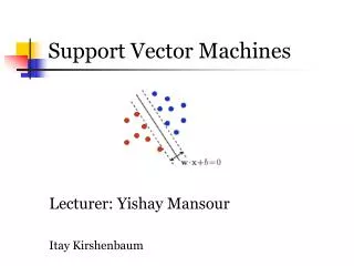
Here, assume positive and negative instances are to be separated by the hyperplane Equation of line: x2 x1
Intuition: the best hyperplane (for future generalization) will “maximally” separate the examples
Definition of Margin Vapnik (1979) showed that the hyperplane maximizing the margin of S will have minimal VC dimension in the set of all consistent hyperplanes, and will thus be optimal.
Definition of Margin Vapnik (1979) showed that the hyperplane maximizing the margin of S will have minimal VC dimension in the set of all consistent hyperplanes, and will thus be optimal. This is an optimization problem!
Note that the hyperplane is defined as • To make the math easier, we will rescale w and b such that the hyperplane is halfway in-between the closest positive and negative examples, and
Geometry of the Margin (www.svms.org/tutorials/Hearst-etal1998.pdf) -
In this case, the margin is • So to maximize the margin, we need to minimize .
Minimizing ||w|| Find w and b by doing the following minimization: This is a quadratic optimization problem. Use “standard optimization tools” to solve it.
Dual formulation: It turns out that w can be expressed as a linear combination of a small subset of the training examples xi: those that lie exactly on margin (minimum distance to hyperplane): such that xi lie exactly on the margin. • These training examples are called “support vectors”. They carry all relevant information about the classification problem.
The results of the SVM training algorithm (involving solving a quadratic programming problem) are the i and the bias b. • The support vectors are all xi such that i > 0.
For a new example x, We can now classify x using the support vectors: • This is the resulting SVM classifier.
SVM review • Equation of line: w1x1 + w2x2 + b = 0 • Define margin using: • Margin distance: • To maximize the margin, we minimize ||w|| • subject to the constraint that positive examples • fall on one side of the margin, and negative • examples on the other side: • We can relax this constraint using “slack variables”
SVM review • To do the optimization, we use the dual formulation: • The results of the optimization “black box” are • and b . • The support vectors are all xisuch that i!= 0.
SVM review • Once the optimization is done, we can classify a new • example x as follows: • That is, classification is done entirely through a linear • combination of dot products with training examples. • This is a “kernel” method.
Example 2 1 1 2 -2 -1 -1 -2
Example Input to SVM optimzer: x1 x2 class 1 1 1 1 2 1 2 1 1 -1 0 -1 0 -1 -1 -1 -1 -1 2 1 1 2 -2 -1 -1 -2
Example Input to SVM optimzer: x1 x2 class 1 1 1 1 2 1 2 1 1 -1 0 -1 0 -1 -1 -1 -1 -1 Output from SVM optimzer: Support vectorα (-1, 0) -.208 (1, 1) .416 (0, -1) -.208 b = -.376 2 1 1 2 -2 -1 -1 -2
Example Input to SVM optimzer: x1 x2 class 1 1 1 1 2 1 2 1 1 -1 0 -1 0 -1 -1 -1 -1 -1 Output from SVM optimzer: Support vectorα (-1, 0) -.208 (1, 1) .416 (0, -1) -.208 b = -.376 2 1 1 2 -2 -1 Weight vector: -1 -2
Example Input to SVM optimzer: x1 x2 class 1 1 1 1 2 1 2 1 1 -1 0 -1 0 -1 -1 -1 -1 -1 Output from SVM optimzer: Support vectorα (-1, 0) -.208 (1, 1) .416 (0, -1) -.208 b = -.376 2 1 1 2 -2 -1 Weight vector: -1 -2 Separation line:
Example 2 1 1 2 -2 -1 -1 Classifying a new point: -2
Non-linearly separable training examples • What if the training examples are not linearly separable?
Non-linearly separable training examples • What if the training examples are not linearly separable? • Use old trick: find a function that maps points to a higher dimensional space (“feature space”) in which they are linearly separable, and do the classification in that higher-dimensional space.
x2 Need to find a function that will perform such a mapping: : n F Then can find hyperplane in higher dimensional feature space F, and do classification using that hyperplane in higher dimensional space. x2 x1 x1 x3
Example Find a 3-dimensional feature space in which XOR is linearly separable. x2 x2 (0, 1) (1, 1) (1, 0) x1 x3 (0, 0) x1
Problem: • Recall that classification of instance x is expressed in terms of dot products of x and support vectors. • The quadratic programming problem of finding the support vectors and coefficients also depends only on dot products between training examples, rather than on the training examples outside of dot products.
So if each xi is replaced by (xi) in these procedures, we will have to calculate (xi) for each i as well as calculate a lot of dot products, (xi)(xj) • But in general, if the feature space F is high dimensional, (xi) (xj) will be expensive to compute.
Second trick: • Suppose that there were some magic function, k(xi, xj) = (xi) (xj) such that k is cheap to compute even though (xi) (xj) is expensive to compute. • Then we wouldn’t need to compute the dot product directly; we’d just need to compute k during both the training and testing phases. • The good news is: such k functions exist! They are called “kernel functions”, and come from the theory of integral operators.
Example: Polynomial kernel: Suppose x = (x1, x2) andz= (z1,z2).
Example Does the degree-2 polynomial kernel make XOR linearly separable? (0, 1) (1, 1) x2 (1, 0) (0, 0) x1
Recap of SVM algorithm Given training set S = {(x1, y1), (x2, y2), ..., (xm, ym) | (xi, yi)n{+1, -1} • Choose a map : nF, which maps xi to a higher dimensional feature space. (Solves problem that X might not be linearly separable in original space.) • Choose a cheap-to-compute kernel function k(x,z)=(x) (z) (Solves problem that in high dimensional spaces, dot products are very expensive to compute.)
Apply quadratic programming procedure (using the kernel function k) to find a hyperplane (w,b), such that where the (xi)’s are support vectors, the i’s are coefficients, andbis a bias, such that (w, b) is the hyperplane maximizing the margin of the training set in feature space F.
5. Now, given a new instance, x, find the classification of x by computing