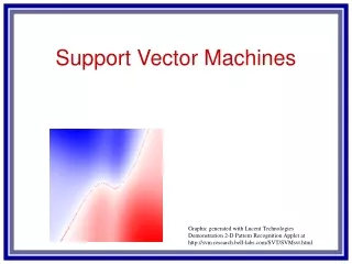
Support Vector Machines
Support Vector Machines. RBF-networks Support Vector Machines Good Decision Boundary Optimization Problem Soft margin Hyperplane Non-linear Decision Boundary Kernel-Trick Approximation Accurancy Overtraining. Gaussian response function. Each hidden layer unit computes

Support Vector Machines
E N D
Presentation Transcript
RBF-networks • Support Vector Machines • Good Decision Boundary • Optimization Problem • Soft margin Hyperplane • Non-linear Decision Boundary • Kernel-Trick • Approximation Accurancy • Overtraining
Gaussian response function • Each hidden layer unit computes • x = an input vector • u = weight vector of hidden layer neuron i
Location of centers u • The location of the receptive field is critical • Apply clustering to the training set • each determined cluster center would correspond to a center u of a receptive field of a hidden neuron
Determining • Following heuristic will perform well in practice • For each hidden layer neuron, find the RMS distance between ui and the center of its N nearest neighbors cj • Assign this value to i
The output neuron produces the linear weighted sum • The weights have to be adopted • (LMS)
f( ) f( ) f( ) f( ) f( ) f( ) f( ) f( ) f( ) f( ) f( ) f( ) f( ) f( ) f( ) f( ) Why does a RBF network work? • The hidden layer applies a nonlinear transformation from the input space to the hidden space • In the hidden space a linear discrimination can be performed
Support Vector Machines • Linear machine • Constructs a hyperplane as the decision surface in such a way that the margin of separation between positive and negative examples is maximized • Good generalization performance • Support vector learning algorithm may construct following three learning machines • Polynominal learning machines • Radial-Basis functions networks • Two-layer perceptrons
Two Class Problem: Linear Separable Case • Many decision boundaries can separate these two classes • Which one should we choose? Class 2 Class 1
Example of Bad Decision Boundaries Class 2 Class 2 Class 1 Class 1
Good Decision Boundary: Margin Should Be Large • The decision boundary should be as far away from the data of both classes as possible • We should maximize the margin, m w/||w|| * (x1-x2) = 2/||w|| Class 2 m Class 1
The Optimization Problem • Let {x1, ..., xn} be our data set and let yi {1,-1} be the class label of xi • The decision boundary should classify all points correctly • A constrained optimization problem
The Optimization Problem • Introduce Lagrange multipliers , • Lagrange function: • Minimized with respect to w and b
The Optimization Problem • We can transform the problem to its dual • This is a quadratic programming (QP) problem • Global maximum of ai can always be found • w can be recovered by
A Geometrical Interpretation a10=0 Class 2 a8=0.6 a7=0 a2=0 a5=0 a1=0.8 a4=0 a6=1.4 a9=0 a3=0 Class 1
How About Not Linearly Separable • We allow “error” xi in classification Class 2 Class 1
Soft Margin Hyperplane • Define xi=0 if there is no error for xi • xi are just “slack variables” in optimization theory • We want to minimize • C : tradeoff parameter between error and margin • The optimization problem becomes
The Optimization Problem • The dual of the problem is • w is also recovered as • The only difference with the linear separable case is that there is an upper bound C on ai • Once again, a QP solver can be used to find ai
Extension to Non-linear Decision Boundary • Key idea: transform xi to a higher dimensional space to “make life easier” • Input space: the space xi are in • Feature space: the space of f(xi) after transformation • Why transform? • Linear operation in the feature space is equivalent to non-linear operation in input space • The classification task can be “easier” with a proper transformation. Example: XOR
f( ) f( ) f( ) f( ) f( ) f( ) f( ) f( ) f( ) f( ) f( ) f( ) f( ) f( ) f( ) f( ) f( ) f( ) Extension to Non-linear Decision Boundary • Possible problem of the transformation • High computation burden and hard to get a good estimate • SVM solves these two issues simultaneously • Kernel tricks for efficient computation • Minimize ||w||2 can lead to a “good” classifier f(.) Feature space Input space
Example Transformation • Define the kernel function K (x,y) as • Consider the following transformation • The inner product can be computed by K without going through the map f(.)
Kernel Trick • The relationship between the kernel function K and the mapping f(.) is • This is known as the kernel trick • In practice, we specify K, thereby specifying f(.) indirectly, instead of choosing f(.) • Intuitively, K (x,y) represents our desired notion of similarity between data x and y and this is from our prior knowledge • K (x,y) needs to satisfy a technical condition (Mercer condition) in order for f(.) to exist
Examples of Kernel Functions • Polynomial kernel with degree d • Radial basis function kernel with width s • Closely related to radial basis function neural networks • Sigmoid with parameter k and q • It does not satisfy the Mercer condition on all k and q • Research on different kernel functions in different applications is very active
Multi-class Classification • SVM is basically a two-class classifier • One can change the QP formulation to allow multi-class classification • More commonly, the data set is divided into two parts “intelligently” in different ways and a separate SVM is trained for each way of division • Multi-class classification is done by combining the output of all the SVM classifiers • Majority rule • Error correcting code • Directed acyclic graph
Conclusion • SVM is a useful alternative to neural networks • Two key concepts of SVM: maximize the margin and the kernel trick • Many active research is taking place on areas related to SVM • Many SVM implementations are available on the web for you to try on your data set!
Measuring Approximation Accuracy • Comparing its output with correct values • Mean squared Error F(w) of the network • D={(x1,t1),(x2,t2), . .,(xd,td),..,(xm,tm)}
RBF-networks • Support Vector Machines • Good Decision Boundary • Optimization Problem • Soft margin Hyperplane • Non-linear Decision Boundary • Kernel-Trick • Approximation Accurancy • Overtraining
Bibliography • Simon Haykin, Neural Networks, Secend edition Prentice Hall, 1999