Support Vector Machines
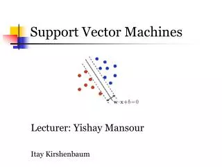
Support Vector Machines. Perceptron Revisited:. y( x ) = sign( w . x + b ). Linear Classifier:. w . x + b > 0. w . x + b = 0. w . x + b < 0. Which one is the best?. d. Notion of Margin. Distance from a data point to the boundary:


Support Vector Machines
E N D
Presentation Transcript
Perceptron Revisited: y(x) = sign(w.x + b) • Linear Classifier: w.x + b > 0 w.x + b = 0 w.x + b < 0
d Notion of Margin • Distance from a data point to the boundary: • Data points closest to the boundary are called support vectors • Margindis the distance between two classes. r
Maximum Margin Classification • Intuitively, the classifier of the maximum margin is the best solution • Vapnik formally justifies this from the view of Structure Risk Minimization • Also, it seems that only support vectors matter (is SVM a statistical classifier?)
Quantifying the Margin: • Canonical hyper-planes: • Redundancy in the choice of w and b: • To break this redundancy, assuming the closest data points are on the hyper-planes (canonical hyper-planes): • The margin is: • The condition of correct classification w.xi+ b≥ 1 if yi= 1 w.xi+ b ≤ -1 if yi= -1
Maximizing Margin: • The quadratic optimization problem: • A simpler formulation: Find w and b such that is maximized; and for all {(xi,yi)} w.xi+ b≥ 1 if yi=1; w.xi+ b ≤ -1 if yi= -1
The dual problem (1) • Quadratic optimization problems are a well-known class of mathematical programming problems, and many (rather intricate) algorithms exist for solving them. • The solution involves constructing a dual problem: • The Lagrangian L: • Minimizing L over w and b:
The dual problem (2) • Therefore, the optimal value of w is: • Using the above result we have: • The dual optimization problem
Important Observations (1): • The solution of the dual problem depends on the inner-product between data points, i.e., rather than data points themselves. • The dominant contribution of support vectors: • The Kuhn-Tucker condition • Only support vectors have non-zero h values
Important Observations (2): • The form of the final solution: • Two features: • Only depending on support vectors • Depending on the inner-product of data vectors • Fixing b:
Soft Margin Classification • What if data points are not linearly separable? • Slack variablesξican be added to allow misclassification of difficult or noisy examples. ξi ξi
The formulation of soft margin • The original problem: • The dual problem:
Linear SVMs: Overview • The classifier is a separating hyperplane. • Most “important” training points are support vectors; they define the hyperplane. • Quadratic optimization algorithms can identify which training points xi are support vectors with non-zero Lagrangian multipliers hi. • Both in the dual formulation of the problem and in the solution training points appear only inside inner-products.
x 0 x 0 Who really need linear classifiers • Datasets that are linearly separable with some noise, linear SVM work well: • But if the dataset is non-linearly separable? • How about… mapping data to a higher-dimensional space: x2 x 0
Non-linear SVMs: Feature spaces • General idea: the original space can always be mapped to some higher-dimensional feature space where the training set becomes separable: Φ: x→φ(x)
The “Kernel Trick” • The SVM only relies on the inner-product between vectors xi.xj • If every datapoint is mapped into high-dimensional space via some transformation Φ: x→φ(x), the inner-product becomes: K(xi,xj)= φ(xi).φ(xj) • K(xi,xj ) is called the kernel function. • For SVM, we only need specify the kernel K(xi,xj ), without need to know the corresponding non-linear mapping, φ(x).
Non-linear SVMs • The dual problem: • Optimization techniques for finding hi’s remain the same! • The solution is:
Examples of Kernel Trick (1) • For the example in the previous figure: • The non-linear mapping • The kernel • Where is the benefit?
Examples of Kernel Trick (2) • Polynomial kernel of degree 2 in 2 variables • The non-linear mapping: • The kernel
Examples of kernel trick (3) • Gaussian kernel: • The mapping is of infinite dimension: • The moral: very high-dimensional and complicated non-linear mapping can be achieved by using a simple kernel!
What Functions are Kernels? • For some functions K(xi,xj) checking that K(xi,xj)= φ(xi).φ(xj) can be cumbersome. • Mercer’s theorem: Every semi-positive definite symmetric function is a kernel
Examples of Kernel Functions • Linear kernel: • Polynomial kernel of power p: • Gaussian kernel: • In the form, equivalent to RBFNN, but has the advantage of that the center of basis functions, i.e., support vectors, are optimized in a supervised. • Two-layer perceptron:
SVM Overviews • Main features: • By using the kernel trick, data is mapped into a high-dimensional feature space, without introducing much computational effort; • Maximizing the margin achieves better generation performance; • Soft-margin accommodates noisy data; • Not too many parameters need to be tuned. • Demos(http://svm.dcs.rhbnc.ac.uk/pagesnew/GPat.shtml)
SVM so far • SVMs were originally proposed by Boser, Guyon and Vapnik in 1992 and gained increasing popularity in late 1990s. • SVMs are currently among the best performers for many benchmark datasets. • SVM techniques have been extended to a number of tasks such as regression [Vapnik et al. ’97]. • Most popular optimization algorithms for SVMs are SMO [Platt ’99] and SVMlight[Joachims’ 99], both use decomposition to handle large size datasets. • It seems the kernel trick is the most attracting site of SVMs. This idea has now been applied to many other learning models where the inner-product is concerned, and they are called ‘kernel’ methods. • Tuning SVMs remains to be the main research focus: how to an optimal kernel? Kernel should match the smooth structure of data.