Support Vector Machines

1. Support Vector Machines Chapter 12

2. Separating Hyperplanes – Separable Case Extension to Non-separable case – SVM Nonlinear SVM SVM as a Penalization method SVM regression Outline

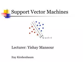
3. Separating Hyperplanes • The separating hyperplane with maximum margin is likely to perform well on test data. • Here the separating hyperplane is almost identical to the more standard linear logistic regression boundary

4. Distance to Hyperplanes • For any point x0 in L, • βT x0 = -β0 • The signed distance of any point x to L is given by

5. MaximumMargin Classifier • Found by quadratic programming (Convex optimization) • Solution determined by just a few points (support vectors) near the boundary • Sparse solution in dual space • Decision function

6. Non-separable Case: Standard Support Vector Classifier This problem computationally equivalent to

7. Computation of SVM • Lagrange (prime) function: • Minimize w.r.t , 0 and i, a set derivatives to zero:

8. Computation of SVM • Lagrange (dual) function: with constraints: 0 I and i=1iyi = 0 • Karush-Kuhn-Tucker conditions:

9. Computation of SVM • The final solution:

10. Example-Mixture Data

11. SVMs for large p, small n • Suppose we have 5000 genes(p) and 50 samples(n), divided into two classes • Many more variables than observations • Infinitely many separating hyperplanes in this feature space • SVMs provide the unique maximal margin separating hyperplane • Prediction performance can be good, but typically no better than simpler methods such as nearest centroids • All genes get a weight, so no gene selection • May overfit the data

12. Non-Linear SVM via Kernels • Note that the SVM classifier involves inner products <xi, xj>=xiTxj • Enlarge the feature space • Replacing xiT xj by appropriate kernel K(xi,xj) = <(xi), (xj)> provides a non-linear SVM in the input space

13. Popular kernels

14. Kernel SVM-Mixture Data

15. Radial Basis Kernel • Radial Basis function has infinite-dim basis: (x) are infinite dimension. • Smaller the Bandwidth c, more wiggly the boundary and hence Less overlap • Kernel trick doesn’t allow coefficients of all basis elements to be freely determined

16. SVM as penalization method • For , consider the problem • Margin Loss + Penalty • For , the penalized setup leads to the same solution as SVM.

17. SVM and other Loss Functions

18. Population Minimizers for Two Loss Functions

19. Logistic Regression with Loglikelihood Loss

20. Curse of Dimensionality in SVM

21. SVM Loss-Functions for Regression

22. Example

23. Example

24. Example

25. Generalized Discriminant Analysis Chapter 12

26. Outline • Flexible Discriminant Analysis(FDA) • Penalized Discriminant Analysis • Mixture Discriminant Analysis (MDA)

27. Linear Discriminant Analysis • Let P(G = k) = k and P(X=x|G=k) = fk(x) • Then • Assume fk(x) ~ N(k, k) and 1 =2 = …=K= • Then we can show the decision rule is (HW#1):

28. LDA (cont) • Plug in the estimates:

29. LDA Example Prediction Vector Data In this three class problem, the middle class is classified correctly

30. LDA Example 11 classes and X  R10

31. Virtues and Failings of LDA • Simple prototype (centriod) classifier • New observation classified into the class with the closest centroid • But uses Mahalonobis distance • Simple decision rules based on linear decision boundaries • Estimated Bayes classifier for Gaussian class conditionals • But data might not be Gaussian • Provides low dimensional view of data • Using discriminant functions as coordinates • Often produces best classification results • Simplicity and low variance in estimation

32. Virtues and Failings of LDA • LDA may fail in number of situations • Often linear boundaries fail to separate classes • With large N, may estimate quadratic decision boundary • May want to model even more irregular (non-linear) boundaries • Single prototype per class may not be insufficient • May have many (correlated) predictors for digitized analog signals. • Too many parameters estimated with high variance, and the performance suffers • May want to regularize

33. Generalization of LDA • Flexible Discriminant Analysis (FDA) • LDA in enlarged space of predictors via basis expansions • Penalized Discriminant Analysis (PDA) • With too many predictors, do not want to expand the set: Already too large • Fit LDA model with penalized coefficient to be smooth/coherent in spatial domain • With large number of predictors, could use penalized FDA • Mixture Discriminant Analysis (MDA) • Model each class by a mixture of two or more Gaussians with different centroids, all sharing same covariance matrix • Allows for subspace reduction

34. Linear regression on derived responses for K-class problem Define indicator variables for each class (K in all) Using indicator functions as responses to create a set of Y variables Flexible Discriminant Analysis • Obtain mutually linear score functions as discriminant (canonical) variables • Classify into the nearest class centroid • Mahalanobis distance of a test point x to kth class centroid

35. Flexible Discriminant Analysis • Mahalanobis distance of a test point x to kth class centroid • We can replace linear regression fits by non-parametric fits, e.g., generalized additive fits, spline functions, MARS models etc., with a regularizer or kernel regression and possibly reduced rank regression

36. Computation of FDA • Multivariate nonparametric regression • Optimal scores • Update the model from step 1 using the optimal scores

37. Example of FDA N(0, I) N(0, 9I/4) Bayes decision boundary FDA using degree-two Polynomial regression

38. Speech Recognition Data • K=11 classes • spoken vowels sound • p=10 predictors extracted from digitized speech • FDA uses adaptive additive-spline regression (BRUTO in S-plus) • FDA/MARS Uses Multivariate Adaptive Regression Splines; degree=2 allows pairwise products

39. LDA Vs. FDA/BRUTO

40. Penalized Discriminant Analysis • PDA is a regularized discriminant analysis on enlarged set of predictors via a basis expansion

41. Penalized Discriminant Analysis • PDA enlarge the predictors to h(x) • Use LDA in the enlarged space, with the penalized Mahalanobis distance: with W as within-class Cov

42. Penalized Discriminant Analysis • Decompose the classification subspace using the penalized metric: max w.r.t.

43. USPS Digit Recognition

44. Digit Recognition-LDA vs. PDA

45. PDA Canonical Variates

46. Mixture Discriminant Analysis • The class conditional densities modeled as mixture of Gaussians • Possibly different # of components in each class • Estimate the centroids and mixing proportions in each subclass by max joint likelihood P(G, X) • EM algorithm for MLE • Could use penalized estimation

47. FDA and MDA

48. Wave Form Signal with Additive Gaussian Noise Class 1: Xj = U h1(j) +(1-U)h2(j) +j Class 2: Xj = U h1(j) +(1-U)h3(j) +j Class 3: Xj = U h2(j) +(1-U)h3(j) +j Where j = 1,L, 21, and U ~ Unif(0,1) h1(j) = max(6-|j-11|,0) h2(j) = h1(j-4) h3(j) = h1(j+4)

49. Wave From Data Results