
Chapter 6 Random Processes
E N D
Presentation Transcript
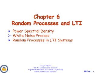
Chapter 6Random Processes • Description of Random Processes • Stationarity and ergodicty • Autocorrelation of Random Processes • Properties of autocorrelation Huseyin Bilgekul EEE 461 Communication Systems II Department of Electrical and Electronic Engineering Eastern Mediterranean University
Homework Assignments • Return date: November 8, 2005. • Assignments: Problem 6-2 Problem 6-3 Problem 6-6 Problem 6-10 Problem 6-11
Random Processes • A RANDOM VARIABLEX, is a rule for assigning to every outcome, w, of an experiment a number X(w). • Note: X denotes a random variable and X(w) denotes a particular value. • A RANDOM PROCESSX(t) is a rule for assigning to every w, a function X(t,w). • Note: for notational simplicity we often omit the dependence on w.
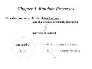
Ensemble of Sample Functions The set of all possible functions is called the ENSEMBLE.
Random Processes • A general Random or Stochastic Process can be described as: • Collection of time functions (signals) corresponding to various outcomes of random experiments. • Collection of random variables observed at different times. • Examples of random processes in communications: • Channel noise, • Information generated by a source, • Interference. t1 t2
Collection of Time Functions • Consider the time-varying function representing a random process where wi represents an outcome of a random event. • Example: • a box has infinitely many resistors (i=1,2, . . .) of same resistance R. • Let wi be event that the ith resistor has been picked up from the box • Let v(t, wi) represent the voltage of the thermal noise measured on this resistor.
Collection of Random Variables • For a particular time t=to the value x(to,wi) is a random variable. • To describe a random process we can use collection of random variables {x(to,w1) , x(to,w2) , x(to,w3) , . . . }. • Type: a random processes can be either discrete-time or continuous-time. • Probability of obtaining a sample function of a RP that passes through the following set of windows. Probability of a joint event.
Description of Random Processes • Analytical description:X(t) =f(t,w) where w is an outcome of a random event. • Statistical description: For any integer N and any choice of (t1, t2, . . ., tN) the joint pdf of {X(t1), X( t2), . . ., X( tN) } is known. To describe the random process completely the PDF f(x) is required.
Example: Analytical Description • Let where q is a random variable uniformly distributed on [0,2p]. • Complete statistical description of X(to)is: • Introduce • Then, we need to transform from y to x: • We need both y1 and y2 because for a given x the equation x=A cos(y) has two solutions in [0,2p].
Analytical (continued) • Note x and y are actual values of the random variables X and Y. • Since and pY is uniform in [2pf0t0, 2pf0t0 + 2p], we get • Using the analytical description of X(t),we obtained its statistical description at any time t.
Example: Statistical Description • Suppose a random process x(t) has the property that for any N and (t0,t1, . . .,tN) the joint density function of {x(ti)}is a jointly distributed Gaussian vector with zero mean and covariance • This gives complete statistical description of the random process x(t).
x(t) x(t) 2 B t t B intersect is Random Activity: Ensembles • Consider the random process: x(t)=At+B • Draw ensembles of the waveforms: • B is constant, A is uniformly distributed between [-1,1] • A is constant, B is uniformly distributed between [0,2] • Does having an “Ensemble” of waveforms give you a better picture of how the system performs? Slope Random
Stationarity • Definition: A random process is STATIONARY to the order N if for any t1,t2, . . . , tN, fx{x(t1), x(t2),...x(tN)}=fx{x(t1+t0), x(t2+t0),...,x(tN +t0)} • This means that the process behaves similarly (follows the same PDF) regardless of when you measure it. • A random process is said to be STRICTLY STATIONARY if it is stationary to the order of N→∞. • Is the random process from the coin tossing experiment stationary?
Illustration of Stationarity Time functions pass through the corresponding windows at different times with the same probability.
Example of First-Order Stationarity • Assume that A and w0 are constants; q0 is a uniformly distributed RV from [-p,p);t is time. • From last lecture, recall that the PDF of x(t): • Note: there is NO dependence on time, the PDF is not a function of t. • The RP is STATIONARY.
Non-Stationary Example • Now assume that A,q0 and w0 are constants; t is time. • Value of x(t) is always known for any time with a probability of 1. Thus the first order PDF of x(t) is • Note: The PDF depends on time, so it is NONSTATIONARY.
Ergodic Processes • Definition: A random process is ERGODIC if all time averages of any sample function are equal to the corresponding ensemble averages (expectations) • Example, for ergodic processes, can use ensemble statistics to compute DC values and RMS values • Ergodic processes are always stationary; Stationary processes are not necessarily ergodic
Example: Ergodic Process • A and w0 are constants; q0 is a uniformly distributed RV from [-p,p);t is time. • Mean (Ensemble statistics) • Variance
Example: Ergodic Process • Mean (Time Average) T is large • Variance • The ensemble and time averages are the same, so the process is ERGODIC
EXERCISE • Write down the definition of : • Wide sense stationary • Ergodic processes • How do these concepts relate to each other? • Consider: x(t) = K; K is uniformly distributed between [-1, 1] • WSS? • Ergodic?
Autocorrelation of Random Process • The Autocorrelation function of a real random process x(t) at two times is:
Wide-sense Stationary • A random process that is stationary to order 2 or greater is Wide-Sense Stationary: • A random process is Wide-Sense Stationaryif: • Usually, t1=t and t2=t+tso that t2- t1 =t. • Wide-sense stationary process does not DRIFT with time. • Autocorrelation depends only on the time gap but not where the time difference is. • Autocorrelation gives idea about the frequency response of the RP.
Autocorrelation Function of RP • Properties of the autocorrelation function of wide-sense stationary processes Autocorrelation of slowly and rapidly fluctuating random processes.
Cross Correlations of RP • Cross Correlation of two RP x(t) and y(t) is defined similarly as: • If x(t) and y(t) are Jointly Stationary processes, • If the RP’s are jointly ERGODIC,
Cross Correlation Properties of Jointly Stationary RP’s • Some properties of cross-correlation functions are • Uncorrelated: • Orthogonal: • Independent: if x(t1) and y(t2) are independent (joint distribution is product of individual distributions)