Download
1 / 35
350 likes | 366 Vues
Explore the class of covariance functions, including isotropic correlations and the popular squared exponential function, and learn about spectral representation and estimation methods.

E N D
NRCSE 2. Covariances
Valid covariance functions • The class of covariance functions is the class of positive definite functions C: • Why? • Bochner’s theorem: Every positive definite function C continuous at 0,0 can be written • for a finite measure μ on R2. • (Spectral representation)
Spectral representation By the spectral representation any isotropic continuous correlation on Rd is of the form By isotropy, the expectation depends only on the distribution G of . Let Y be uniform on the unit sphere. Then
Isotropic correlation • Jv(u) is a Bessel function of the first kind and order v. • Hence • and in the case d=2 • (Hankel transform)
The Bessel function J0 –0.403
The exponential correlation • A commonly used correlation function is (v) = e–v/. Corresponds to a Gaussian process with continuous but not differentiable sample paths. • More generally, (v) = c(v=0) + (1-c)e–v/ has a nugget c, corresponding to measurement error and spatial correlation at small distances. • All isotropic correlations are a mixture of a nugget and a continuous isotropic correlation.
The squared exponential • Using yields • corresponding to an underlying Gaussian field with analytic paths. • This is sometimes called the Gaussian covariance, for no really good reason. • A generalization is the power(ed) exponential correlation function,
The spherical • Corresponding variogram nugget sill range
The Matérn class • where is a modified Bessel function of the third kind and order . It corresponds to a spatial field with –1 continuous derivatives • =1/2 is exponential; • =1 is Whittle’s spatial correlation; • yields squared exponential.
Estimation of variograms • Recall • Method of moments: square of all pairwise differences, smoothed over lag bins • Problems: Not necessarily a valid variogram • Not very robust
A robust empirical variogram estimator • (Z(x)-Z(y))2 is chi-squared for Gaussian data • Fourth root is variance stabilizing • Cressie and Hawkins:
Least squares • Minimize • Alternatives: • fourth root transformation • weighting by 1/2 • generalized least squares
Maximum likelihood • Z~Nn(,) = [(si-sj;)] = V() • Maximize • and q maximizes the profile likelihood
Asymptotics • Increasing domain asymptotics: let region of interest grow. Station density stays the same • Bad estimation at short distances, but effectively independent blocks far apart • Infill asymptotics: let station density grow, keeping region fixed. • Good estimates at short distances. No effectively independent blocks, so technically trickier
Stein’s result • Covariance functions C0 and C1 are compatible if their Gaussian measures are mutually absolutely continuous. Sample at {si, i=1,...,n}, predict at s (limit point of sampling points). Let ei(n) be kriging prediction error at s for Ci, and V0 the variance under C0 of some random variable. • If limnV0(e0(n))=0, then
Properties of Fourier transforms • Convolution • Scaling • Translation
Parceval’s theorem • Relates space integration to frequency integration. Decomposes variability.
Spectral representation • Stationary processes • Spectral process Y has stationary increments • If F has a density f, it is called the spectral density.
Estimating the spectrum • For process observed on nxn grid, estimate spectrum by periodogram • Equivalent to DFT of sample covariance
Properties of the periodogram • Periodogram values at Fourier frequencies (j,k)are • uncorrelated • asymptotically unbiased • not consistent • To get a consistent estimate of the spectrum, smooth over nearby frequencies
Some common isotropic spectra • Squared exponential • Matérn
Thetford canopy heights • 39-year thinned commercial plantation of Scots pine in Thetford Forest, UK • Density 1000 trees/ha • 36m x 120m area surveyed for crown height • Focus on 32 x 32 subset
Spectrum of canopy heights 72-76° ridge Row effect
Global processes • Problems such as global warming require modeling of processes that take place on the globe (an oriented sphere). Optimal prediction of quantities such as global mean temperature need models for global covariances. • Note: spherical covariances can take values in [-1,1]–not just imbedded in R3. • Also, stationarity and isotropy are identical concepts on the sphere.
Isotropic covariances on the sphere Isotropic covariances on a sphere are of the form where p and q are directions, pq the angle between them, and Pi the Legendre polynomials. Example: ai=(2i+1)ri
Global temperature • Global Historical Climatology Network 7280 stations with at least 10 years of data. Subset with 839 stations with data 1950-1991 selected.