Download
1 / 63
650 likes | 844 Vues
Reminder - Means, Variances and Covariances. Covariance Algebra. Covariance and Correlation. Correlation is covariance scaled to range [-1,1]. For two traits with the same variance: Cov(X 1 ,X 2 ) = r 12 Var(X). Phenotypes, Genotypes and environment.

E N D
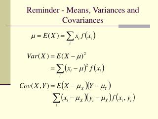
Covariance and Correlation Correlation is covariance scaled to range [-1,1]. For two traits with the same variance: Cov(X1,X2) = r12 Var(X)
Phenotypes, Genotypes and environment • A phenotype (P) is composed of genotypic values (G) and environmental deviations (E): P = G + E • Whether we focus on mean, variance, or covariance, inference always comes from the measurement of the phenotype • A distinction will be made: • V will be used to indicate inferred components of variance • s2will be used to indicate observational components of variance • Mean genotypic value is equal to the mean phenotypic value • Genotypic values are expressed as deviations from the mid-homozygote point E(Gj) = E(Pj )= mPj
Genotypic values • Consider two alleles, A1 and A2, at a single locus. • The two homozygous classes, A1A1 and A2A2, are assigned genotypic values +a and -a, respectively. • Assume that the A1 allele increases the value of a phenotype while the A2 allele decreases the value. • The heterozygous class, A1A2, is assigned a genotypic value of d • Zero is midpoint between the two genotypic values of A1A1 and A2A2; d is measured as a deviation from this midpoint
Genotype A2A2 A1A2 A1A1 -a 0 d +a Genotypic value
Properties of the Genotypic Values and Environmental Deviations • The mean of environmental deviations is zero Ej = Pj – Gj , ,(mE = 0) • The correlation between genotypic values and environmental deviations for a population of subjects is zero (rGE = .00)
Population mean mP = mG = SGkpk • Multiply frequency by genotypic value and sum • Recall that p2 - q2 = (p + q)(p - q) = p - q mP = a(p - q) + 2dpq
Additive model • Assume aA and aB correspond to A1A1 and B1B1 • A1A1B1B1 = aA+ aB • So that mP=Sa(p - q) +2Sdpq
Average effect for an allele (a) • Population properties vis a vis family structure • Transmission from parent to offspring; parents pass on genes and not genotypes • Average effect of a particular gene (allele) is the mean deviation from the population mean of individuals which received that gene from one parent (assuming the gene transmitted from the other parent having come at random from the population)
Average effect for an allele (a) • Thus, the average effect for each allele also can be calculated for A1 and A2 in the following manner (Falconer, 1989): a1 = pa + qd - [a(p - q) + 2dpq] and a2 = -p[a + d(q - p)]
Average effect of a gene substitution • Assume two alleles at a locus • Select A2 genes at random from population; p in A1A2 and q in A2A2 • A1A2 to A1A1 corresponds to a change of d to +a, i.e., (a - d); A2A2 to A1A2 corresponds to a change of -a to d, (d + a) • On average, p(a - d) plus q(d + a) or a = a + d(q - p)
Breeding Value (A) • The average effects of the parents’ genes determine the mean genotypic value of its progeny • Average effect can not be measured (gene substitution), while breeding value can • Breeding value: Value of individual compared to mean value of its progeny • Mate with a number of random partners; breeding value equals twice the mean deviation of the progeny from the population mean (provides only half the genes) • Breeding value is interpretable only when we know in which population the individual is to be mated
Breeding Value • Genotype: Breeding value A1A1: 2a1 = 2qa A1A2: a1 + a2 = (q - p)a A2A2: 2a2 = -2pa • Mean breeding value under HWC equilibrium is zero 2p2qa + 2pq(q - p)a - 2q2pa which equals... 2pqa(p + q - p - q) = 0
Dominance deviation • Breeding values are referred to as “additive genotype”; variation due to additive effects of genes • A symbolizes the breeding value of an individual • Proportion of s2P attributable to s2A is called heritability (h2) G = A + D • Statistically speaking, within-locus interaction • Non-additive, within-locus effect • A parent can not individually transmit dominance effects; it requires the gametic contribution of both parents
Genotypic values, breeding values, and dominance deviation 2qa +a d 0 (q - p)a }a 0 -2pa -a Genotypic values Breeding values A2A2 A1A2 A1A1 q2 2pq p2
Genotypic values, breeding values, and dominance deviation • Regression of genotypic value on gene dosage yields the genotypic values predicted by gene dosage • average effect of an allele • that which “breeds true” • If there is dominance, this prediction of genotypic values from gene dosage will be slightly off • dominance is deviation from the regression line
Epitasis - Separate analysis • locus A shows an association with the trait • locus B appears unrelated Locus B Locus A
Epitasis - Joint analysis • locus B modifies the effects of locus A
Genotypic Means Locus A Locus BAA Aa aa BBAABBAaBBaaBBBB BbAABbAaBbaaBbBb bbAabbAabbaabbbb AAAaaa
Partitioning of effects • Locus A • Locus B M P M P
4 main effects M Additive effects P M P
6 twoway interactions M M P P Additive-additive epistasis M P M P
4 threeway interactions M P M Additive-dominance epistasis P P M M P M M P P
1 fourway interaction Dominance-dominance epistasis M P M P
m m m – aA + aA – aa + aB + aB + da + dA + aa + aB m m m + aA – aA + dB + ad + dA + dB + dd + dB – ad m m m – aA – aB – aa – da – aB – aB + aA + dA + aa Two loci AA Aa aa BB Bb bb
Covariance matrix Sib 1 Sib 2 Sib 1 2A + 2D + 2S + 2N2A + z2D+ 2S Sib 2 2A + z2D+ 2S2A + 2D + 2S + 2N Sib 1 Sib 2 Sib 1 2A + 2D + 2S + 2N½2A + ¼2D+ 2S Sib 2 ½2A + ¼2D+ 2S2A + 2D + 2S + 2N
Detecting epistasis • The test for epistasis is based on the difference in fit between • - a model with single locus effects and epistatic effects and • - a model with only single locus effects, • Enables us to investigate the power of the variance components method to detect epistasis
True Model Assumed Model A B A a a* b Y Y a* is the apparent co-efficient a* will deviate from a to the extent that A and B are correlated
Phenotypic variance • Again, assume P = G + E • Thus differences in phenotypes, measured as variance and symbolized as VP, can be decomposed into both genetic and environmental variation, VG and VE, respectively. VP= VG + VE • VG is comprised of three kinds of distinct variance: additive (VA), dominant (VD), and epistatic (VI). VP= (VA +VD + VI ) + VE
Additive (VA) and dominance variance (VD) • The covariance between breeding values and dominance deviations equals zero so that VG= VA + VD + VI VA=2pq[a + d(q - p)]2 VD = d2(4q4p2 + 8p3q3 + 4p4q2) = (2pqd)2
Additive and dominance variance • If d = 0, then VA=2pqa2, where q is the recessive allele • If d = a, then VA= 8pq3a2 • If p = q = .50 (e.g., cross of two inbred strains) • VA=1/2a2 • VD=1/4d2 • In general, genes at intermediate frequency contribute more variance than high or low frequencies
Epistatic variance (VI) • Epistatic variance beyond three or more loci do not contribute substantially to total variance • Three types of two-factor interactions (breeding values by dominance deviations) • additive x additive (VAA) • additive x dominance (VAD) • dominance x dominance (VDD)
Environmental variance • Special environmental variance (VEs) • within-individual component • temporary or localized circumstance • General environmental variance (VEg) • between-individual component • permanent or non-localized circumstances • Ratio of between-individual to total phenotypic is an intraclass correlation (r)
Components of variance - Summary Phenotypic Variance Environmental Genetic GxE interaction and correlation
Components of variance - Summary Phenotypic Variance Environmental Genetic GxE interaction Additive Dominance Epistasis and correlation
Components of variance - Summary Phenotypic Variance Environmental Genetic Additive Dominance Epistasis Quantitative trait loci GxE interaction and correlation
Resemblance of relatives • Degree of relative resemblance is a function of additive variance, i.e, breeding values • The proportionate amount of additive variance is an estimate of heritability (VA / VP) • Intraclass correlation coefficient t = s2B / s2B + s2W • Between and within full-sibships, for example
Resemblance of relatives bOP = CovOP / s2P • New property of the population is covariance of related individuals
Cross-Products of Deviations for Pairs of Relatives AA Aa aa AA (a-m)2 Aa (a-m)(d-m) (d-m)2 aa (a-m)(-a-m) (-a-m)(d-m) (-a-m)2 The covariance between relatives of a certain class is the weighted average of these cross-products, where each cross-product is weighted by its frequency in that class.
Offspring and one parent • Individual genotypic values and those of their offspring produced by random mating • When expressed as normal deviations, the mean value of the offspring is 1/2 the breeding value of the parent • Covariance between individual’s genotypic value (G) with 1/2 its breeding value (A)
Covariance for Parent-offspring (P-O) AA Aa aa AA p3 Aa p2q pq aa 0 pq2 q3 Covariance = (a-m)2p3 + (d-m)2pq + (-a-m)2q3 + (a-m)(d-m)2p2q+ (-a-m)(d-m)2pq2 = pq[a+(q-p)d]2 = VA / 2
Offspring and one parent • G = A + D so that covariance is between (A + D) and 1/2A; sum of cross products equal S1/2A(A + D) = 1/2SA2 + 1/2SAD • CovOP = (1/2SA2 + 1/2SAD) / # of parents • Recall that CovAD = 0 • CovOP = 1/2VA (i.e., 1/2 the variance of breeding values)
Offspring and one parent • Mean genotypic values of the offspring are 1/2A of the parents • Mean cross product equals Frequency X Genotypic value of the parent X Mean genotypic value of the offspring • CovOP = pqa2(p2+2pq+q2)+2p2q2ad(-q+q-p+p)=pqa2=1/2VA • (Note: VA = 2pqa2)