IV. Neural Network Learning
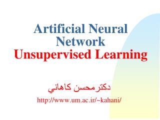
IV. Neural Network Learning. A. Neural Network Learning. Supervised Learning. Produce desired outputs for training inputs Generalize reasonably & appropriately to other inputs Good example: pattern recognition Feedforward multilayer networks. input layer. output layer. hidden layers.

IV. Neural Network Learning
E N D
Presentation Transcript
Supervised Learning • Produce desired outputs for training inputs • Generalize reasonably & appropriately to other inputs • Good example: pattern recognition • Feedforward multilayer networks
input layer output layer hidden layers Feedforward Network . . . . . . . . . . . . . . . . . .
connectionweights inputs Typical Artificial Neuron output threshold
linearcombination activationfunction net input(local field) Typical Artificial Neuron
Net input: Neuron output: Equations
Single-Layer Perceptron . . . . . .
Variables x1 w1 h S Q y xj wj wn xn q
w2 x f w1 v 2D Weight Vector – + w
N-Dimensional Weight Vector + normal vector w separating hyperplane –
Goal of Perceptron Learning • Suppose we have training patterns x1, x2, …, xP with corresponding desired outputs y1, y2, …, yP • where xp {0, 1}n, yp {0, 1} • We want to find w, q such thatyp = Q(wxp – q) for p = 1, …, P
Treating Threshold as Weight x1 w1 h S Q y xj wj wn xn q
x0 = = w0 Treating Threshold as Weight –1 x1 q w1 h S Q y xj wj wn xn
Adjustment of Weight Vector z5 z1 z10 z9 z11 z8 z6 z2 z3 z4 z7
Outline ofPerceptron Learning Algorithm • initialize weight vector randomly • until all patterns classified correctly, do: • for p = 1, …, P do: • if zp classified correctly, do nothing • else adjust weight vector to be closer to correct classification
Perceptron Learning Theorem • If there is a set of weights that will solve the problem, • then the PLA will eventually find it • (for a sufficiently small learning rate) • Note: only applies if positive & negative examples are linearly separable
NetLogo Simulation of Perceptron Learning Run Perceptron-Geometry.nlogo
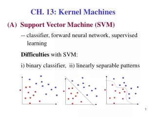
Classification Power of Multilayer Perceptrons • Perceptrons can function as logic gates • Therefore MLP can form intersections, unions, differences of linearly-separable regions • Classes can be arbitrary hyperpolyhedra • Minsky & Papert criticism of perceptrons • No one succeeded in developing a MLP learning algorithm
. . . input layer output layer hidden layers Credit Assignment Problem How do we adjust the weights of the hidden layers? Desired output . . . . . . . . . . . . . . . . . .
NetLogo Demonstration ofBack-Propagation Learning Run Artificial Neural Net.nlogo
Control Algorithm C Adaptive System Evaluation Function (Fitness, Figure of Merit) System S F … … P1 Pk Pm Control Parameters
F gradient ascent Gradient Ascenton Fitness Surface + –
Gradient Ascent Process Therefore gradient ascent increases fitness (until reaches 0 gradient)
Recap The Jacobian depends on the specific form of the system, in this case, a feedforward neural network
Multilayer Notation WL–1 xq yq W1 WL–2 W2 s1 sL s2 sL–1
Notation • L layers of neurons labeled 1, …, L • Nl neurons in layer l • sl = vector of outputs from neurons in layer l • input layer s1 = xq (the input pattern) • output layer sL = yq (the actual output) • Wl = weights between layers l and l+1 • Problem: find how outputs yiq vary with weights Wjkl (l = 1, …, L–1)
Typical Neuron s1l–1 Wi1l–1 Wijl–1 hil S s sjl–1 sil WiNl–1 sNl–1
Output-Layer Neuron s1L–1 Wi1L–1 WijL–1 hiL S s sjL–1 tiq siL = yiq WiNL–1 Eq sNL–1
Hidden-Layer Neuron s1l s1l–1 s1l+1 W1il Wi1l–1 Wijl–1 Wkil hil S s sjl–1 skl+1 Eq sil WiNl–1 WNil sNl–1 sNl+1 sNl