Introduction to Graph Theory: Concepts, Implementation, and Key Terminology
This document covers the foundational concepts of graph theory, including types of graphs, terminology, and implementation techniques. It introduces directed and undirected graphs, adjacency matrices, and lists, and provides insights on trees and forests. The exploration of properties, paths, cycles, and connectivity lays the groundwork for understanding complex networks. Examples from transportation and computer networks illustrate real-world applications, while insights into implementation strategies highlight considerations for dense versus sparse graphs.

Introduction to Graph Theory: Concepts, Implementation, and Key Terminology
E N D
Presentation Transcript
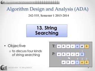
Algorithm Design and Analysis (ADA) 242-535, Semester 1 2013-2014 • Objective • introduce the main kinds of graphs, discuss two implementation approaches, and remind you about trees 8. Introduction to Graphs
Overview • Graphs • Graph Terminology • Implementing Graphs • adjency matrix • adjency list • Trees and Forests • Tree Terminology
1. Graphs • A graph has two parts (V, E), where: • V are the nodes, called vertices • E are the links between vertices, called edges • Example: • airports and distance between them 849 PVD 1843 ORD 142 SFO 802 LGA 1743 337 1387 HNL 2555 1099 1233 LAX 1120 DFW MIA
1.1.Graph Types • Directedgraph • the edges are directed • e.g., bus cost network • Undirectedgraph • the edges are undirected • e.g., road network
1.2. Examples • Electronic circuits • Printed circuit board • Integrated circuit • Transportation networks • Highway network • Flight network • Computer networks • Local area network • Internet • Web • Databases • Entity-relationship diagram
A Calling Graph • A calling graph for a program: main makeList printList mergeSort 4 examples of recursion split merge
Sheet Metal Hole Drilling • Problem: minimise the moving time of the drill over a metal sheet. continued
A Weighted Graph Version • Add edge numbers (weights) for the movement time between any two holes. 8 b a 6 2 6 4 c 3 d 5 9 12 4 e
2. Graph Terminology V a b h j U d X Z c e i W g f Y • End vertices (or endpoints) of an edge • U and V are the endpoints • Edges incident on a vertex • a, d, and b are incident • Adjacent vertices • U and V are adjacent • Degree of a vertex • X has degree 5 • Parallel edges • h and i are parallel edges • Self-loop • j is a self-loop
Path • sequence of alternating vertices and edges • begins with a vertex • ends with a vertex • each edge is preceded and followed by its endpoints • Simple path • path such that all its vertices and edges are distinct • Examples • P1=(V,b,X,h,Z) is a simple path • P2=(U,c,W,e,X,g,Y,f,W,d,V) is a path that is not simple V b a P1 d U X Z P2 h c e W g f Y
Cycle • circular sequence of alternating vertices and edges • each edge is preceded and followed by its endpoints • Simple cycle • cycle such that all its vertices and edges are distinct • Examples • C1=(V,b,X,g,Y,f,W,c,U,a) is a simple cycle • C2=(U,c,W,e,X,g,Y,f,W,d,V,a,) is a cycle that is not simple V a b d U X Z C2 h e C1 c W g f Y Graphs
Connectivity • A graph is connected if there is a path between every pair of vertices Connected graph Non connected graph with two connected components
Some Properties Property Sv degree(v)= 2*| E | Proof: each undirected edge is counted twice(called the handshaking lemma) Property In an undirected graph with no self-loops and no multiple edges |E| |V| (|V| -1)/2 Proof: each vertex has degree at most (|V| -1) Notation Vset of vertices Eset of edges |. . .| the set size degree()degree of a vertex c Example • | V | = 4 • | E | = 6 • degree(a)= 3 d b a
3. Implementing Graphs • We will typically express running times in terms of |E| and |V| (often dropping the |’s) • If |E| |V|2 the graph is dense • can also write this as |E| is O(|v2|) • If |E| |V| the graph is sparse • or |E| is O(|V|) • Dense and sparse graphs are best implemented using two different data structures: • Adjacency matricies: for dense graphs • Adjacency lists: for sparse graphs
Dense Big-Oh • In the most dense graph, a graph of vverticies will have |V|(|V|-1)/2 edges. • In that case, for large n, |E|is O(|V|2) |V| = 5 |E| = (5*4)/2 = 10
Proof that a graph of n nodes has n(n-1)/2 edges. Write as S(n) = n(n-1)/2 • Basis. S(2) = 1. True. • Inductive Case. • assume S(n) = n(n-1)/2 (1) • try to show S(n+1) = (n+1)n/2 (2) • we know: S(n+1) = S(n) + n which is • S(n+1) = n(n-1)/2 + n which is • S(n+1) = (n+1)n/2 which is (2)
3.1. Adjacency Matrix a b a b c d e a 0 1 0 0 1 b 1 0 1 0 1 c 0 1 1 0 1 c d 0 0 0 0 1 e 1 1 1 1 0 d e Graph Adjacency Matrix
Properties • An adjacency matrixrepresents the graph as a V * Vmatrix A: • A[i, j] = 1 if edge (i, j) E = 0 if edge (i, j) E • The degree of a vertex v (of a simple graph) = sum of row v or sum of column v • e.g. vertexa has degree 2 since it is connected to b and e • An adjacency matrix can represent loops • e.g. vertex c on the previous slide continued
An adjacency matrix can represent parallel edgesif non-negative integers are allowed as matrix entries • ijth entry = no. of edges between vertex i and j • The matrix duplicates information around the main diagonal • the size can be easily reduced with some coding tricks • Properties of graphs can be obtained using matrix operations • e.g. the no. of paths of a given length, and vertex degree
The No. of Paths of Length n • If an adjacency matrix A is multiplied by itself repeatedly: • A, A2, A3, ..., An Then the ijth entry in matrix An is equal to the number of paths from i to j of length n.
Example a b a b c d e A = a 0 1 0 1 0 b 1 0 1 0 1 c c 0 1 0 1 1 d 1 0 1 0 0 e 0 1 1 0 0 d e
a b c d e 0 1 0 1 0 0 1 0 1 0 a 2 0 2 0 1 1 0 1 0 1 1 0 1 0 1 b 0 3 1 2 1 A2 = = c 0 1 0 1 1 0 1 0 1 1 2 1 3 0 1 1 0 1 0 0 1 0 1 0 0 d 0 2 0 2 1 0 1 1 0 0 0 1 1 0 0 e 1 1 1 1 2
Why it Works... • Consider row a, column c in A2: c a-b-c b d 0 a-d-c ( 0 1 0 1 0 ) a 1 b = 0*0 + 1*1 + 0*0 + 1*1 + 0*1= 2 0 d 1 1 continued
A non-zero product means there is at least one vertex connecting verticiesa and c. • The sum is 2 because of: • (a, b, c) and (a, d, c) • 2 paths of length two
The Degree of Verticies • The entries on the main diagonal of A2 give the degrees of the verticies (when A is a simple graph). • Consider vertex c: • degree of c == 3 since it is connected to the edges (c,b), (c,d), and (c,e). continued
In A2 these become paths of length 2: • (c,b,c), (c,d,c), and (c,e,c) • So the number of paths of length 2 for c = the degree of c • this is true for all verticies
Coding Adjacency Matricies • #define NUMNODESnint arcs[NUMNODES][NUMNODES]; • arcs[u][v] == 1 if there is an edge (u,v); 0 otherwise • Storage used: O(|V|2) • The implementation may also need a way to map node names (strings) to array indicies. continued
If n is large then the array will be very large, with almost half of it being unnecessary. • If the nodes are lightly connected then most of the array will contain 0’s, which is a further waste of memory.
Representing Directed Graphs • A directed graph: 0 1 3 2 4
Its Adjacency Matrix • Not symmetric; all the array may be necessary. • Still a waste of space if nodes are lightly connected. finish 0 1 2 3 4 0 1 1 1 0 0 0 0 0 1 0 1 2 1 1 0 0 1 start 0 0 1 0 1 3 0 1 0 0 0 4
When to use an Adjacency Matrix • The adjacency matrix is an efficient way to store dense graphs. • But most large interesting graphs are sparse • e.g., planar graphs, in which no edges cross, have |e| = O(|v|) by Euler’s formula • For this reason the adjacency list is often a better respresentation than the adjacency matrix
Euler’s Formula Characteristic • Euler (1752) proved that for any connected graph, where: F = no. of facesE = no. of edgesV = no. of verticies/nodes then the formula holds: F = E – V + 2 F = 5; E = 9; V = 6
3.2. Adjacency List • Adjacency list: for each vertex v V, store a list of vertices adjacent to v • Example: • adj[0] = {0, 1, 2} • adj[1] = {3} • adj[2] = {0, 1, 4} • adj[3] = {2, 4} • adj[4] = {1} • Can be used for directed and undirected graphs. 0 1 3 2 4
0 1 0 1 2 4 3 1 4 2 • An implementation diagram: adj[] 0 1 2 3 means NULL size of array = no. of vertices (|V|) 4 no. of cells == no. of edges (|E|)
Data Structures • struct cell { /* for a linked list */ Node nodeName; struct cell *next;};struct cell *adj[NUMNODES]; • adj[u] points to a linked list of cells which give the names of the nodes connected to u.
Storage Needs • How much storage is required? • The degree of a vertex v == number of incident edges • directed graphs have in-degree, out-degree values • For directed graphs, the number of items in an adjacency lists is out-degree(v) = |E| • This uses (V + E) storage
For undirected graphs, the number of items in the adjency list is degree(v) = 2*|E| (the handshaking lemma) • Why? If we mark every edge connected to every vertex, then by the end, every edge will be marked twice • This also uses (V + E) storage • In summary, adjacency lists use (V+E) storage
3.3. Running Time: Matrix or List? • Which representation is better for graphs? • The simple answer: • dense graph – use a matrix • sparse graph – use an adjcency list • But a more accurate answer depends on the operations that will be applied to the graph. • We will consider three operations: • is there an edge between u and v? • find the successors of u (in a directed graph) • find the predecessors of u (in a directed graph) continued
Is there an edge (u,v)? • Adjacency matrix: O(1) to read arcs[u][v] • Adjacency list: O(1 + E/V) // forget the |...| • O(1) to get to adj[u] • length of linked list is on average E/V • if a sparse graph (E<<V): O(1+ E/V) => O(1) • if a dense graph (E ≈ V2): O(1+ E/V) => O(V)
Find u’s successors (u->v) • Adjacency matrix: O(V) since must examine the entire row for vertex u • Adjacency list: O(1 + (E/V)) since must look at entire list pointed to by adj[u] • if a sparse graph (E<<V): O(1+ E/V) => O(1) • if a dense graph (E ≈ V2): O(1+ E/V) => O(V)
Find u’s predecessors (t->u) • Adjacency matrix: O(V) since must examine the entire column for vertex u • a 1 in the row for ‘t’ means that ‘t’ is a predecessor • Adjacency list: O(E) since must examine every list pointed to by adj[] • if a sparse graph (E<<V): O(E) is fast • if a dense graph (E ≈ V2): O(E) is slow
Summary: which is faster? • Operation Dense Graph Sparse GraphFind edge Adj. Matrix EitherFind succ. Either Adj. listFind pred. Adj. Matrix Either • As a graph gets denser, an adjacency matrix has better execution time than an adjacency list.
3.4. Storage Space: Matrix or List? • The size of an adjacency matrix for a graph of V nodes is: • V2 bits (assuming 0 and 1 are stored as bits) continued
An adjacency list cell uses: • 32 bits for the integer, 32 bits for the pointer • so, cell size = 64 bits • Total no. of cells = total no. of edges, e • so, total size of lists = 64*E bits • successors[] has V entries (for V verticies) • so, array size is 32*V bits • Total size of an adjacency list data struct: 64*E + 32*V
Size Comparison • An adjacency list will use less storage than an adjacency matrix when: 64*E + 32*V < V2 which is: E < V2/64 – V/2 When V is large, ignore the V/2 term: E < V2/64 continued
V2 is (roughly) the maximum number of edges. • So if the actual number of edges in a graph is 1/64 of the maximum number of edges, then an adj. list representation will be smaller than an adj. matrix coding • but the graph must be quite sparse
4. Trees and Forests • A (free) tree is an undirected graph T such that • T is connected • T has no cycles This definition of tree is different from the one of a rooted tree • A forest is an undirected graph without cycles • The connected components of a forest are trees Tree Forest Graphs
Uses of Trees President Vice-President for Academics Vice-President for Admin. Dean of Engineering Dean of Business Planning Officer Purchases Officer . . . . . . . . Head of CoE Head of EE Head of AC. . . . .
Saturated Hydrocarbons H • Non-rooted (free) trees • a free tree is a graph with no cycles H H H C H H C C C H H C H H H C H H H C H H Isobutane H C H H Butane H