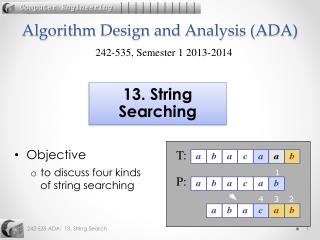
Graph Search Algorithms: Depth-First and Breadth-First Techniques

1. Algorithm Design and Analysis (ADA) 242-535, Semester 1 2013-2014 • Objective • describe and compare depth-first and breadth-first graph searching, and look at the creation of spanning trees 9. Graph Search

2. Overview • Graph Searching • Depth First Search (DFS) • Uses of DFS • cycle detection, reachability, topological sort • Breadth-first Search (BFS) • DFS vs. BFS • IP Multicasting

3. 1. Graph Searching • Given: a graph G = (V, E), directed or undirected • Goal: visit every vertex • Often the end result is a tree built over the graph • called a spanning tree • it visits every vertex, but not necessarily every edge • Pick any vertex as the root • Choose certain edges to produce a tree • Note: we might build a forest if the graph is not connected

4. Example search then build a spanning tree(or trees)

5. 2. Depth First Search (DFS) • DFS is “depth first” because it always fully explores down a path away from a vertex v before it looks at other paths leaving v. • Crucial DFS properties: • uses recursion: essential for graph structures • choice: at a vertex there may be a choice of several edges to follow to the next vertex • backtracking: "return to where you came from" • avoid cycles by grouping vertices into visited and unvisited

6. Directed Graph Example a DFS works with directed and undirected graphs. b d e f c Graph G

7. Data Structures • enum MARKTYPE {VISITED, UNVISITED};struct cell { /* adj. list */NODE nodeName; struct cell *next;};typedef struct cell *LIST;struct graph { enum MARKTYPE mark; LIST successors;};typedef struct graph GRAPH[NUMNODES];

8. The dfs() Function void dfs(NODE u, GRAPH G)// recursively search G, starting from u{ LIST p; // runs down adj. list of u NODE v; // node in cell that p points at G[u].mark = VISITED; // visited u p = G[u].successors; while (p != NULL) { // visit u’s succ’s v = p->nodeName; if (G[v].mark == UNVISITED)dfs(v, G); // visit v p = p->next; }}

9. Calling dfs(a,G) call it d(a) for short • Call Visitedd(a) {a}d(a)-d(b) {a,b}d(a)-d(b)-d(c) {a,b,c} Skip b, return to d(b)d(a)-d(b)-d(d) {a,b,c,d} Skip cd(a)-d(b)-d(d)-d(e) {a,b,c,d,e} Skip c, return to d(d) continued

10. d(a)-d(b)-d(d)-d(f) {a,b,c,d,e,f} Skip c, return to d(d)d(a)-d(b)-d(d) {a,b,c,d,e,f} Return to d(b)d(a)-d(b) {a,b,c,d,e,f} Return to d(a)d(a) {a,b,c,d,e,f} Skip d, return

11. DFS Spanning Tree • Since nodes are marked, the graph is searched as if it were a tree: A spanning treeis a subgraph of a graph Gwhich contains all the verticies of G. a/1 b/2 d/4 c/3 e/5 f/6 c

12. Example 2 a a b b c d c d e f e f DFS h h g g the tree generated by DFS isdrawn withthick lines

13. dfs() Running Time • The time taken to search from a node is proportional to the no. of successors of that node. • Total search time for all nodes = O(|V|)Total search time for all successors = time to search all edges = O(|E|) • Total running time is O(V + E) continued

14. If the graph is dense, E >> V(E approaches V2) then the O(V)term can be ignored • in that case, the total running time = O(E) or O(V2)

15. 3. Uses of DFS • Finding cycles in a graph • e.g. for finding recursionin a call graph • Searching complex locations, such as mazes • Reachability detection • i.e. can a vertex v be reached from vertex u? • useful for e-mail routing; path finding • Strong connectivity • Topological sorting continued

16. Maze Traversal • The DFS algorithm is similar to a classic strategy for exploring a maze • mark each intersection, corner and dead end (vertex) as visited • mark each corridor (edge ) traversed • keep track of the path back to the previous branch points Graphs

17. Reachability • DFS tree rooted at v: what are the vertices reachable from v via directed paths? E D C start at C E D A C F E D A B C F A B start at B

18. a g c d e b f Strong Connectivity • Each vertex can reach all other vertices Graphs

19. Strong Connectivity Algorithm • Pick a vertex v in G. • Perform a DFS from v in G. • If there’s a vertex not visited, print “no”. • Let G’ be G with edges reversed. • Perform a DFS from v in G’. • If there’s a vertex not visited, print “no” • If the algorithm gets here, print “yes”. • Running time: O(V+E). a G: g c d e b f a g G’: c d e b f

20. a g c d e b f Strongly Connected Components • List all the subgraphs where each vertex can reach all the other vertices in that subgraph. • Can also be done in O(V+E)time using DFS. { a , c , g } { f , d , e , b }

21. Topological Sort • Topological sort of a directed acyclic graph (DAG): • linearly order all the vertices in a graph G such that vertex u comes before vertex v if edge (u, v)  G • a DAG is a directed graph with no directed cycles

22. Example: Getting Dressed Underwear Socks Watch Trousers Shoes Shirt Belt Tie one topological sort (not unique) Jacket Socks Underwear Trousers Shoes Watch Shirt Belt Tie Jacket

23. Topological Sort Algorithm Topological-Sort() { Run DFS; When a vertex is finished, output it; Vertices are output in reverse topological order; } • Time: O(V+E)

24. 4. Breadth-first Search (BFS) • Process all the verticies at a given level before moving to the next level. • Example graph G (again): a b c d e f h g

25. Informal Algorithm • 1) Put the verticies into an ordering • e.g. {a, b, c, d, e, f, g, h} • 2) Select a vertex, add it to the spanning tree T: e.g. a • 3) Add to T all edges (a,X) and X verticies that do not create a cycle in T • i.e. (a,b), (a,c), (a,g) T = {a, b, c, g} a g b c continued

26. a • Repeat step 3 on the verticies just added, these are on level 1 • i.e. b: add (b,d) c: add (c,e) g: nothing T = {a,b,c,d,e} • Repeat step 3 on the verticies just added, these are on level 2 • i.e. d: add (d,f) e: nothing T = {a,b,c,d,e,f} level 1 g b c d e a g b c level 2 d e f continued

27. a • Repeat step 3 on the verticies just added, these are on level 3 • i.e. f: add (f,h) T = {a,b,c,d,e,f,h} • Repeat step 3 on the verticies just added, these are on level 4 • i.e. h: nothing, so stop g b c d e level 3 f h continued

28. Resulting spanning tree: a b a different spanning tree from the earlier solution c d e f h g

29. Example 2

30. Algorithm Graphically pre-built adjency list start node

33. BFS Code boolean marked[]; // visited this vertex? int edgeTo[]; // vertex number going to this vertex void bfs(Graph graph, int start) { Queue q = new Queue(); marked[start] = true; q.add(start); // add to end of queue while (!q.isEmpty()) { int v = q.remove(); // get from start of queue for (int w : graph.adjacentTo(v)) // v --> w if (!marked[w]) { edgeTo[w] = v; // save last edge on a shortest path marked[w] = true; q.add(w); // add to end of queue } } } // end of bfs()

34. 5. DFS vs. BFS see part 11

35. DFS and BFS as Maze Explorers • DFS is like one person exploringa maze • do down a path to the end, get to a dead-end, backtrack, and try a different path • BFS is like a group of searchers fanning out in all directions, each unrolling a ball of string. • at a branch point, the searchers split up to explore all the branches at once • if two groups meet up, they join forces (using the ball of string of the group that got there first) • the group that gets to the exit first has found the shortest path

36. BFS Maze Graphically Also called flood filling; used in paint software.

37. Sequential / Parallel • The BFS "fanning out" algorithm is best implemented in a parallel language, where each "group of explorers" is a separate thread of execution. • e.g. use fork and join in Java • The earlier implementation uses a queue to implement the fanning out as a sequential algorithm. • DFS is inherently a sequential algorithm.

38. 6. IP Multicasting • A network of computers and routers: source computer router continued

39. How can a packet (message) be sent from the source computer to every other computer? • The inefficient way is to use broadcasting • send a copy along every link, and have each router do the same • each router and computer will receive many copies of the same packet • loops may mean the packet never disappears! continued

40. IP multicasting is an efficient solution • send a single packet to one router • have the router send it to 1 or more routers in such a way that a computer never receives the packet more than once • This behaviour can be represented by a spanning tree. • Can use either BFS or DFS, but BFS will usually produce shorter paths • i.e. BFS is a better choice continued

41. One spanning tree for the network: source computer the tree is drawn with thick lines router