Download
1 / 71
710 likes | 864 Vues
This presentation by Shaun Purcell and Pak Sham explores the concept of power in QTL linkage analysis, emphasizing the importance of hypothesis testing, statistical significance, and interpretation of results. It discusses types of errors in decision-making (Type I and Type II errors), the role of p-values, and the implications of significant versus non-significant findings. Practical exercises illustrate how to calculate power in genetic studies, using chi-squared tests to evaluate allele frequencies and their correlation with traits. The ultimate goal is to enhance confidence in findings and improve experimental design.

E N D
Power in QTL linkage analysis Shaun Purcell & Pak Sham SGDP, IoP, London, UK F:\pshaun\power.ppt
YES NO Test statistic Power primer • Statistics (e.g. chi-squared, z-score) are continuous measures of support for a certain hypothesis YES OR NO decision-making : significance testing Inevitably leads to two types of mistake : false positive (YES instead of NO) (Type I) false negative (NO instead of YES) (Type II)
Hypothesis testing • Null hypothesis : no effect • A ‘significant’ result means that we can reject the null hypothesis • A ‘nonsignificant’ result means that we cannot reject the null hypothesis
Statistical significance • The ‘p-value’ • The probability of a false positive error if the null were in fact true • Typically, we are willing to incorrectly reject the null 5% or 1% of the time (Type I error)
Misunderstandings • p - VALUES • that the p value is the probability of the null hypothesis being true • that high p values mean large and important effects • NULL HYPOTHESIS • that nonrejection of the null implies its truth
Limitations • IF A RESULT IS SIGNIFICANT • leads to the conclusion that the null is false • BUT, this may be trivial • IF A RESULT IS NONSIGNIFICANT • leads only to the conclusion that it cannot be concluded that the null is false
Alternate hypothesis • Neyman & Pearson (1928) • ALTERNATE HYPOTHESIS • specifies a precise, non-null state of affairs with associated risk of error
Sampling distribution if H0 were true Sampling distribution if HA were true Critical value P(T) T
STATISTICS Nonrejection of H0 Rejection of H0 Type I error at rate Nonsignificant result H0 true R E A L I T Y Type II error at rate Significant result HA true POWER =(1- )
Power • The probability of rejection of a false null-hypothesis • depends on • - the significance crtierion () • - the sample size (N) • - the effect size (NCP) “The probability of detecting a given effect size in a population from a sample of size N, using significance criterion ”
Critical value Impact of alpha P(T) T
Critical value Impact of effect size, N P(T) T
Applications • POWER SURVEYS / META-ANALYSES • - low power undermines the confidence that can be placed in statistically significant results • EXPERIMENTAL DESIGN • - avoiding false positives vs. dealing with false negatives • MAGNITUDE VS. SIGNIFICANCE • - highly significant very important • INTERPRETING NONSIGIFICANT RESULTS • - nonsignficant results only meaningful if power is high
Practical Exercise 1 • Calculation of power for simple case-control association study. • DATA : allele frequency of “A” allele for cases and controls • TEST : 2-by-2 contingency table : chi-squared • (1 degree of freedom)
Step 1 : determine expected chi-squared • Hypothetical allele frequencies • Cases P(A) = 0.68 • Controls P(A) = 0.54 • Sample 150 cases, 150 controls • Excel spreadsheet : faculty drive:\pshaun\chisq.xls Chi-squared statistic = 12.36
Step 2. Determine the critical value for a given type I error rate, - inverse central chi-squared distribution P(T) Critical value T
http://workshop.colorado.edu/~pshaun/gpc/pdf.html • df = 1 , NCP = 0 • X • 0.05 • 0.01 • 0.001 3.84146 6.63489 10.82754
Step 3. Determine the power for a given critical value and non-centrality parameter - non-central chi-squared distribution P(T) Critical value T
Determining power • df = 1 , NCP = 12.36 • X Power • 0.05 3.84146 • 0.01 6.6349 • 0.001 10.827 0.94 0.83 0.59
Exercises • Using the spreadsheet and the chi-squared calculator, what is power (for the 3 levels of alpha) • 1. … if the sample size were 300 for each group? • 2. … if allele frequencies were 0.24 and 0.18 for 750 cases and 750 controls?
Answers • 1. NCP = 24.72 Power • 0.05 1.00 • 0.01 0.99 • 0.001 0.95 • 2. NCP = 16.27 Power • 0.05 0.98 • 0.01 0.93 • 0.001 0.77 • nb. Stata : di 1-nchi(df,NCP,invchi(df,))
POWER Allele frequencies Genetic values Type I errors Type II errors Sample N Effect Size Variance explained QTL linkage
Power of tests • For chi-squared tests on large samples, power is determined by non-centrality parameter () and degrees of freedom (df) • = E(2lnL1 - 2lnL0) • = E(2lnL1 ) - E(2lnL0) • where expectations are taken at asymptotic values of maximum likelihood estimates (MLE) under an assumed true model
Linkage test • HA • H0 for i=j for ij for i=j for ij
Expected log likelihood under H0 Expectation of the quadratic product is simply s, the sibship size (note: standarised trait)
For sib-pairs under complete marker information Determinant of 2-by-2 standardised covariance matrix = 1 - r2 Linkage test Expected NCP
Approximation of NCP NCP per sib pair is proportional to - the # of pairs in the sibship (large sibships are powerful) - the square of the additive QTL variance (decreases rapidly for QTL of v. small effect) - the sibling correlation (structure of residual variance is important)
Allele frequencies Genetic values Recombination fraction QTL linkage POWER Type I errors Type II errors Sample N Effect Size Variance explained Marker vs functional variant
Incomplete linkage • The previous calculations assumed analysis was performed at the QTL. • - imagine that the test locus is not the QTL • but is linked to it. • Calculate sib-pair IBD distribution at the QTL, conditional on IBD at test locus, • - a function of recombination fraction
at QTL 0 1/2 1 at M 0 1/2 1
P(M=0 | QTL) r VS VA / 2 + VS VA + VD + VS + VS VA / 2 + VS + VA + VD + VS • Use conditional probabilities to calculate the sib correlation conditional on IBD sharing at the test marker. For example : for IBD 0 at marker : at QTL 0 1/2 1 C0 =
If the QTL is additive, then • attenuation of the NCP is by a factor of (1-2)4 • = square of the correlation • between the proportions of alleles IBD • at two loci with recombination fraction
Comparison to H-E • Amos & Elston (1989) H-E regression • - 90% power (at significant level 0.05) • - QTL variance 0.5 • - marker and major gene are completely linked • 320 sib pairs • 778 sib pairs if = 0.1
GPC input parameters • Proportions of variance • additive QTL variance • dominance QTL variance • residual variance (shared / nonshared) • Recombination fraction ( 0 - 0.5 ) • Sample size & Sibship size ( 2 - 5 ) • Type I error rate • Type II error rate
GPC output parameters • Expected sibling correlations • - by IBD status at the QTL • - by IBD status at the marker • Expected NCP per sibship • Power • - at different levels of alpha given sample size • Sample size • - for specified power at different levels of alpha given power
From GPC • Modelling additive effects only • Sibships Individuals • Pairs 265 (320) 530 • Pairs ( = 0.1) 666 (778) 1332 Trios ( = 0.1) 220 660 Quads ( = 0.1) 110 440 Quints ( = 0.1) 67 335
Practical Exercise 2 • What is the effect on power to detect linkage of : • 1. QTL variance? • 2. residual sibling correlation? • 3. marker-QTL recombination fraction?
Effect of residual correlation • QTL additive effects account for 10% trait variance • Sample size required for 80% power (=0.05) • No dominance • = 0.1 • A residual correlation 0.35 • B residual correlation 0.50 • C residual correlation 0.65
Selective genotyping Unselected Proband Selection EDAC Maximally Dissimilar ASP Extreme Discordant EDAC Mahanalobis Distance
Selective genotyping • The power calculations so far assume an unselected population. • - calculate expected NCP per sibship • If we have a sample with trait scores • - calculate expected NCP for each sibship conditional on trait values • - this quantity can be used to rank order the sample for genotying
Sibship NCP 1.6 1.4 1.2 1 0.8 0.6 0.4 0.2 0 4 3 2 1 -4 0 -3 Sib 2 trait -1 -2 -1 -2 0 1 -3 2 Sib 1 trait 3 -4 4 Sibship informativeness : sib pairs
Sibship NCP Sibship NCP 2 2 1.5 1.5 1 1 0.5 0.5 0 4 0 Sibship NCP 3 2 4 1 2 3 -4 0 -3 2 Sib 2 trait -1 -2 1.5 1 -1 -2 0 -4 0 1 1 -3 -3 2 Sib 1 trait Sib 2 trait -2 -1 3 -4 -1 0.5 4 -2 0 1 -3 2 0 Sib 1 trait 3 -4 4 4 3 2 1 -4 0 -3 Sib 2 trait -1 -2 -1 -2 0 1 -3 2 Sib 1 trait 3 -4 4 Sibship informativeness : sib pairs dominance rare recessive unequal allele frequencies
Selective genotyping SEL T ASP PS ED EDAC MaxD MDis SEL B p d/a .5 15.82 0 .1 0 17.10 .25 15.45 0 .1 16.88 1 .25 15.76 1 .5 1 18.89 .75 27.64 1 43.16 .9 1