Introduction to Linkage and QTL mapping
370 likes | 635 Vues
Introduction to Linkage and QTL mapping. Sarah Medland. Aim of QTL mapping…. LOCALIZE and then IDENTIFY a locus that regulates a trait (QTL) Locus: Nucleotide or sequence of nucleotides with variation in the population, with different variants associated with different trait levels.

Introduction to Linkage and QTL mapping
E N D
Presentation Transcript
Introduction to Linkage and QTL mapping Sarah Medland
Aim of QTL mapping… LOCALIZE and then IDENTIFY a locus that regulates a trait (QTL) • Locus: Nucleotide or sequence of nucleotides with variation in the population, with different variants associated with different trait levels. • Linkage • localize region of the genome where a QTL that regulates the trait is likely to be harboured • Family-specific phenomenon: Affected individuals in a family share the same ancestral predisposing DNA segment at a given QTL • Association • identify a QTL that regulates the trait • Population-specific phenomenon: Affected individuals in a population share the same ancestral predisposing DNA segment at a given QTL
Genotypic similarity – basic principals • Loci that are close together are more likely to be inherited together than loci that are further apart • Loci are likely to be inherited in context – ie with their surrounding loci • Because of this, knowing that a loci is transmitted from a common ancestor is more informative than simply observing that it is the same allele
Genotypic similarity between relatives IBSAlleles shared Identical By State “look the same”, may have the same DNA sequence but they are not necessarily derived from a known common ancestor - focus for association M3 M1 M2 M3 Q3 Q1 Q2 Q4 IBDAlleles shared Identical By Descent are a copy of the same ancestor allele - focus for linkage M1 M2 M3 M3 Q1 Q2 Q3 Q4 IBD IBS M1 M3 M1 M3 2 1 Q1 Q4 Q1 Q3
In biometrical modeling A is correlated at 1 for MZ twins and .5 for DZ twins • .5 is the average genome-wide sharing of genes between full siblings (DZ twin relationship)
In linkage analysis we will be estimating an additional variance component Q • For each locus under analysis the coefficient of sharing for this parameter will vary for each pair of siblings • The coefficient will be the probability that the pair of siblings have both inherited the same alleles from a common ancestor
MZ=1.0 DZ=0.5 MZ & DZ = 1.0 1 1 1 1 1 1 1 1 Q A C E E C A Q e c a q q a c e PTwin1 PTwin2
DNA polymorphisms • Microsatellites • >100,000 • Many alleles, (CA)n • Very Informative • Not intended to be functional variants • Used in linkage • SNPs • 10,054,521 (25 Jan ‘05) • 10,430,753 (11 Mar ‘06) • Most with 2 alleles (up to 4) • Not very informative • Intended to by functional variants • Used in association or linkage A B
Microsatellite data • Ideally positioned at equal genetic distances across chromosome • Mostly di/tri nucleotide repeats • Raw data consists of allele lengths/calls (bp) • Different primers give different lengths • So to compare data you MUST know which primers were used
Binning • Raw allele lengths are converted to allele numbers or lengths • Example:D1S1646 tri-nucleotide repeat size range130-150 • Logically: Work with binned lengths • Commonly: Assign allele 1 to 130 allele, 2 to 133 allele … • Commercially: Allele numbers often assigned based on reference populations CEPH. So if the first CEPH allele was 136 that would be assigned 1 and 130 & 133 would assigned the next free allele number • Conclusions: whenever possible start from the RAW allele size and work with allele length
Error checking • After binning check for errors • Family relationships (GRR, Rel-pair) • Mendelian Errors (Sib-pair) • Double Recombinants (MENDEL, ASPEX, ALEGRO) • An iterative process
‘Clean’ data • ped file • Family, individual, father, mother, sex, dummy, genotypes • The ped file is used with ‘map’ files to obtain estimates of genotypic sharing between relatives at each of the locations under analysis
Genotypic similarity between relatives IBDAlleles shared Identical By Descent are a copy of the same ancestor allele Pairs of siblings may share 0, 1 or 2 alleles IBD The probability of a pair of relatives being IBD is known as pi-hat M3 M1 M2 M3 Q3 Q1 Q2 Q4 M1 M2 M3 M3 Q1 Q2 Q3 Q4 IBS IBD M1 M3 M1 M3 2 1 Q1 Q4 Q1 Q3
Estimating genotypic sharing… • Output
Identity by Descent (IBD) in sibs • Four parental marker alleles: A-B and C-D • Two siblings can inherit 0, 1 or 2 alleles IBD • IBD 0:1:2 = 25%:50%:25% • Derivation of IBD probabilities at one marker (Haseman & Elston 1972
Distribution of pi-hat • Adult Dutch DZ pairs: distribution of pi-hat at 65 cM on chromosome 19 • < 0.25: IBD=0 group • > 0.75: IBD=2 group • others: IBD=1 group • pi65cat= (0,1,2) • Model resemblance (e.g. correlations, covariances) between sib pairs, or DZ twins, as a function of DNA marker sharing at a particular chromosomal location
Raw Dataset: DutchDZ.rec • DZ twins • Data NInput=18 • Rectangular File= DutchDZ.rec • Labels zyg sex1 age1 med1 ldl1 apob1 lnapoe1 sex2 age2 med2 ldl2 apob2 lnapoe2 ibd0_65 ibd1_65 ibd2_65 pihat65 pi65cat • position 65 on chromosome 19 • ibd0_65 ibd1_65 ibd2_65: probabilities that sibling pair is ibd 0, 1 or 2 • pihat65: pihat estimated as ½(ibd1_65) + (ibd2_65) • pi65cat: sample divided according to π<.25, π>.75 or other • DZ pairs (3 groups according to IBD) only • Estimate FEQ • Test if QTL effect is significant • FEQmodel_DZibd_template.mx
DZ by IBD status Variance = Q + F + E Covariance = πQ + F + E
#define $var ldl !3 variables in the file ldl apob apoe #define nvar 1 #define nvarx2 2 #NGroups 5 G1: Model Parameters Calculation Begin Matrices; X Lower nvar nvar Free ! residual familial pc Z Lower nvar nvar Free ! nonshared env pc T Lower nvar nvar Free ! QTL pc H Full 1 1 End Matrices; Matrix H .5 Start .3 All Begin Algebra; F=X*X'; ! residual familial vc E=Z*Z'; ! nonshared environment vc Q=T*T';! QTL vc End Algebra; Option Rsiduals End Data groups x3 G2: DZ IBD2 twins Data NInput=18 Rectangular File=DutchDZ.rec Labels zyg sex1 age1 med1 t1ldl t1apob t1lnapoe sex2 age2 med2 t2ldl t2apob t2lnapoe ibd0_65 ibd1_65 ibd2_65 pihat65 pi65cat Select if pi65cat =2; Select t1$var t2$var ; Begin Matrices = Group 1; M Full nvar nvarx2 Free K Full 1 1 ! correlation of QTL effects End Matrices; Matrix M 4 4 Matrix K 1 Means M; Covariance F+Q+E | F+K@Q _ F+K@Q | F+Q+E; End Walking through the script…
Covariance Statements G2: DZ IBD2 twins Matrix K 1 Covariance F+Q+E | F+K@Q _ F+K@Q | F+Q+E; G3: DZ IBD1 twins Matrix K .5 Covariance F+Q+E | F+K@Q _ F+K@Q | F+Q+E; G4: DZ IBD0 twins Covariance F+Q+E | F_ F | F+Q+E;
G5: Standardization Calculation Begin Matrices = Group 1; Begin Algebra; V=F+E+Q; ! total variance P=F|E|Q; ! concatenate parameter estimates S=P@V~; ! standardized parameter estimates End Algebra; Label Col P f^2 e^2 q^2 Label Col S f^2 e^2 q^2 !FEQ model Interval S 1 1 - S 1 3 Option Rsiduals Iterations=5000 NDecimals=4 Option Multiple Issat End ! Test for QTL Drop T 1 1 1 Exit Walking through the script…
Converting chi-squares to LOD scores • For univariate linkage analysis (where you have 1 QTL estimate) Χ2/4.6 = LOD
Converting chi-squares to p values • Complicated • Distribution of genotypes and phenotypes • Boundary problems • For univariate linkage analysis (where you have 1 QTL estimate) p(linkage)=
Partition Variance • DZ + MZ pairs • Estimate ACEQ • Test if QTL estimate/significance is different • ACEQmodel_DZibd+MZ.mx
Covariance Statements +MZ G2: DZ IBD2 twins Matrix K 1 Covariance A+C+Q+E | H@A+C+K@Q _ H@A+C+K@Q | A+C+Q+E; G3: DZ IBD1 twins Matrix K .5 Covariance A+C+Q+E | H@A+C+K@Q _ H@A+C+K@Q | A+C+Q+E; G4: DZ IBD0 twins Covariance A+C+Q+E | H@A+C_ H@A+C | A+C+Q+E; G5: MZ twins Covariance A+C+Q+E | A+C+Q _ A+C+Q | A+C+Q+E;
Using the full distribution • More power if we use all the available information • So instead of dividing the sample we will use as a continuous coefficient that will vary between sib-pair across loci
!script for univariate linkage - pihat approach !DZ/SIB #loop $i 1 4 1 #define nvar 1 #NGroups 1 DZ / sib TWINS genotyped Data NInput=324 Missing =-1.0000 Rectangular File=lipidall.dat Labels sample fam ldl1 apob1 ldl2 apob2 … Select apob1 apob2 ibd0m$i ibd1m$i ibd2m$i ; Definition_variables ibd0m$i ibd1m$i ibd2m$i ; Pihat.mx This use of the loop command allows you to run the same script over and over moving along the chromosome The format of the command is: #loop variable start end increment So…#loop $i 1 4 1 Starts at marker 1 goes to marker 4 and runs each locus in turn Each occurrence of $i within the script will be replaced by the current number ie on the second run $i will become 2 With the loop command the last end statement becomes an exit statement and the script ends with #end loop
!script for univariate linkage - pihat approach !DZ/SIB #loop $i 1 4 1 #define nvar 1 #NGroups 1 DZ / sib TWINS genotyped Data NInput=324 Missing =-1.0000 Rectangular File=lipidall.dat Labels sample fam ldl1 apob1 ldl2 apob2 … Select apob1 apob2 ibd0m$i ibd1m$i ibd2m$i ; Definition_variables ibd0m$i ibd1m$i ibd2m$i ; Pihat.mx This use of the ‘definition variables’ command allows you to specify which of the selected variables will be used as covariates The value of the covariate displayed in the mxo will be the values for the last case read
!script for univariate linkage - pihat approach !DZ/SIB #loop $i 1 2 1 #define nvar 1 #NGroups 1 DZ / sib TWINS genotyped Data NInput=324 Missing =-1.0000 Rectangular File=lipidall.dat Labels sample fam ldl1 apob1 ldl2 apob2 … Select apob1 apob2 ibd0m$i ibd1m$i ibd2m$i ; Definition_variables ibd0m$i ibd1m$i ibd2m$i ; Begin Matrices; X Lower nvar nvar free ! residual familial F Z Lower nvar nvar free ! unshared environment E L Full nvar 1 free ! qtl effect Q G Full 1 nvar free ! grand means H Full 1 1 ! scalar, .5 K Full 3 1 ! IBD probabilities (from Merlin) J Full 1 3 ! coefficients 0.5,1 for pihat End Matrices; Specify K ibd0m$i ibd1m$i ibd2m$i Matrix H .5 Matrix J 0 .5 1 Start .1 X 1 1 1 Start .1 L 1 1 1 Start .1 Z 1 1 1 Start .5 G 1 1 1 Pihat.mx
Begin Algebra; F= X*X'; ! residual familial variance E= Z*Z'; ! unique environmental variance Q= L*L'; ! variance due to QTL V= F+Q+E; ! total variance T= F|Q|E; ! parameters in one matrix S= F%V| Q%V| E%V; ! standardized variance component estimates P= ???? ; ! estimate of pihat End Algebra; Labels Row S standest Labels Col S f^2 q^2 e^2 Labels Row T unstandest Labels Col T f^2 q^2 e^2 Means G| G ; Covariance F+E+Q | F+P@Q_ F+P@Q | F+E+Q ; Option NDecimals=4 Option RSiduals Option Multiple Issat !End !test significance of QTL effect ! Drop L 1 1 1 Exit #end loop Pihat.mx You need to fix this before you run the script