QTL Mapping
QTL Mapping. The objectives of this section are: To learn basic concepts related with Quantitative Trait Loci (QTL) analysis, To learn how to use QTL analysis software , To interpret results, and to get acquainted with the various QTL analysis programs and QTL databases .

QTL Mapping
E N D
Presentation Transcript
QTL Mapping • The objectives of this section are: • To learn basic concepts related with Quantitative Trait Loci (QTL) analysis, • To learn how to use QTL analysis software, • To interpret results, and to get acquainted with the various QTL analysis programs and QTL databases. • The focus will be on QTL analysis of self-pollinated plants. However, most of what is covered can be easily extended to cross-pollinated plants, animals, and humans.
Topics • Inheritance of quantitative traits • Identifying trait-linked markers • Single-marker analysis • Interval mapping • Composite interval mapping • Issues in QTL detection • Association mapping • Genomic Selection
Qualitative and Quantitative traits • Qualitative traits: • Phenotypes with discrete and easy to measure values. • Individuals can be correctly classified according to phenotype. • Show mendelian inheritance (monogene) • Little environmental effect • Molecular markers are qualitative traits • Examples: • Quantitative traits: • Individuals cannot be classified by discrete values • Quantitative trait distribution show a continuous range of variation and phenotypes can take any value • Complex mode of inheritance (polygene) • Moderate to great environmental effect) • Examples: Plant height, yield, disease severity, grain weight, etc % of plants 40 20 30 Plant Height (in)
Inheritance of Quantitative traits The study of quantitative trait inheritance followed the same steps as for Mendelian traits. At the beginning they were thought to not follow Mendel’s laws. But it is not true • PARENT 1: • pure line, completely homozygote • 40 inches • PARENT 2: • pure line, completely homozygote • 20 inches F1 F1: range of height distribution but no type of segregation F2: wider range of height distribution but no type of segregation F2
Two genes with additive effect controlling the trait One gene controlling the trait P1 P2 P1 P2 AA X aa AABB X aabb F1 Aa F1 AaBb 50% 50% Frequency Frequency 25% 25% 0 2 1 0 2 3 4 1 No. of favorable alleles No. of favorable alleles 1/16 : AABB 4/16:AaBB + AA Bb 6/16:AaBb + AAbb + aaBB 4/16:aaBb + Aabb 1/16:aabb 1/4: AA 1/2: Aa + aA 1/4: aa
Three genes with additive effect controlling the trait P1 P2 AABBCC X aabbcc F1 AaBb 50% Frequency 25% 4 0 5 2 3 6 1 No. of favorable alleles
Inheritance of Quantitative traits P1 (purple, X very dark red) P2 (white) Going one step further, He saw that within each of the groups there was also some variation aabb AABB AaBb F1(red) Frequency - white + purple Color intensity 1/16 : purple AABB 4/16: dark-red AaBB + AABb 6/16: red AAbb + AaBb + aaBB 4/16: light-red aaBb + Aabb 1/16: white aabb
Inheritance of Quantitative traits Phenotype=Genotype+Environment Then, the distribution of a quantitative trait would follow a normal distribution 4 Frequency 3 2 1 + purple - white Color intensity Analysis of quantitative traits is therefore complicated: Same genotype: 1 and 2 show different phenotype Same phenotype: 1, 3 and 4 is the result of three different genotypes
Inheritance of Quantitative traits The inheritance of quantitative traits also explains the phenomenon of transgressive segregation: In the progeny of a cross we can get phenotypes out of the range of the parents P2 P1 0 10 Frequency Let’s assume 5 loci with additive effects control the trait P1 P2 aabbccddEE X AABBCCDDee Cold tolerance AaBbCcDdEe F1 F2 All possible combinations of alleles at 5 loci. Between them: AABBCCDDEE (all favorable alleles) aabbccddee (all unfavorable alleles)
Inheritance of Quantitative traits Quantitative traits are usually controlled by several genes with small additive effects and influenced by the environment Heritability h2measures the proportion of phenotypic variation (variance) that is due to genetic causes P = G + E; VP = VG + VE A heritability of 40% for cold tolerance means that within that population, genetic differences among individuals are responsible of 40% of the variation. Therefore, 60% is due to environmental causes. However, that does not mean that the cold tolerance of a certain individual is due 40% to genetic causes and 60% to environmental causes. h2 is a property of the population and not of individuals
Inheritance of Quantitative traits Heritability h2measures the proportion of phenotypic variation (variance) that is due to genetic causes P = G + E; VP = VG + VE h2 ranges between 0 and 1 If h2is 0 means : a) The trait is not genetically controlled. All the variation we see is due to environmental factors, or b) The trait is genetically controlled but all individuals have the same genotype h2 is very useful because it allows us to predict the response to artificial selection
Inheritance of Quantitative traits Heritability h2measures the proportion of phenotypic variation (variance) that is due to genetic causes P = G + E; VP = VG + VE h2 is very useful because it allows us to predict the response to artificial selection In plant breeding, the starting point is a segregating population (with genetic variability). The best individuals are selected to be the progenitors of the next generation μ0 Selection differential (S) = μS – μ0 Response to selection (R) = μR – μ0 Realized heritability: Is the ratio of the single-generation progress of selection to the selection differential of the parents. The higher h2, the higher the progress of selection in each generation Frequency μS Grain yield (lb/A) 0 6000 μ0 μR Frequency Grain yield (lb/A) 0 6000
Analysis of Quantitative traits The analysis of quantitative traits is based on the identification of the individual loci (QTL) controlling the trait, their location, effects and interactions A quantitative trait locus/loci (QTL) is the location of individual locus or multiple loci that affects a trait that is measured on a quantitative (linear) scale. These traits are typically affected by more than one gene, and also by the environment. Thus, mapping QTL is not as simple as mapping a single gene that affects a qualitative trait (such as flower color).
Analysis of Quantitative traits There are two main approaches for QTL analysis: a) QTL analysis in mapping populations b) Association mapping Both approaches share a set of common elements: a) A population (array of individuals) that show variability for the trait of study b) Phenotypic information: We need to design an experiment to estimate the phenotypic value of each individual c) Genotypic information: A set of molecular markers that have been run in all the individuals of the population d) A statistical method to estimate QTL position, effects and interactions
Analysis of Quantitative traits QTL analysis in mapping populations We need to develop a population from a single cross between two individuals that show contrasting phenotypes for the trait of study. For example, if we want to study quantitative resistance to Barley Stripe Rust (Pucciniastriiformisf. sp. Hordei) we will develop a population from the cross between a susceptible line and a resistant line. The offspring of that cross will show recombination between the two parents and therefore, some individuals will be resistant and other will be susceptible Different types of mapping populations can be used: Doubled haploids (DH), Recombinant inbred lines (RIL), F2, Back cross (BC), etc. Always all individuals trace back to a single cross
Analysis of Quantitative traits QTL analysis in mapping populations The first step is getting genotypic information for all the individuals of the population: molecular markers P2 P1 Back Cross population P1 P2 High Throughput genotyping platform (SNP)
Analysis of Quantitative traits QTL analysis in mapping populations If molecular markers are polymorphic, we can construct a linkage map based on recombination frequencies:
Maps: Different levels of resolutionMain factors: marker density and population size
y βo 0 x -1 aa AA Genotypic classes Analysis of Quantitative traits QTL analysis in mapping populations The basic QTL analysis method consists in walking trough the chromosomes performing statistical test at the positions of the markers in order to test whether there is a marker-trait association or not - Classify progeny by marker genotype - Compare phenotypic mean between classes (t-test or ANOVA) - Significance = marker linked to QTL - Difference between means = estimate of QTL effect g = (µ1 - µ2)/2 g = genotypic effect µ1 = trait mean for genotypic class AA µ2 = trait mean for genotypic class aa
Marker and QTL unlinked F1 Q A F2 population q a Difference between trait scores of AA and aa is zero. Conclusion: No relationship between trait score (y) and marker genotype (x)
Marker and QTL linked F1 Q A F2 population q a Difference between trait scores of AA and aa is large. Conclusion: Strong relationship between trait score (y) and marker genotype (x)
Analysis of Quantitative traits Disease severity (%) DsT-66 Average Disease severy of plants with allele “A” (Inherited from Resistant parent) = 49.8 Average Disease severity of plants with allele “B” (Inherited from Susceptible parent) = 50.3 49.8 and 50.3 are not statistically different. Therefore, marker DsT-66 is not associated with resitance/susceptibility to the disease
Analysis of Quantitative traits Disease severity (%) ABC261 Average Disease severy of plants with allele “A” (Inherited from Resistant parent) = 30.4 Average Disease severity of plants with allele “B” (Inherited from Susceptible parent) = 69.8 30.4 and 69.8 are statistically different. Therefore, marker ABC261 is linked with a resitance/susceptibility QTL. The additive effect of the QTL is: a = (69.8-30.4)/2 = 14.7