Reverse genetics: Quantitative Trait Locus (QTL) mapping Association mapping
Reverse genetics: Quantitative Trait Locus (QTL) mapping Association mapping. Integrating Mendelian and Quantitative Genetics using molecular techniques. Allele A2. Allele A1. 12. 11. 22. 22. 11. 22. 12. 11. 22. 12. Quantitative trait. 16. 28. 40. 52. 64. 76. 88. Height.

Reverse genetics: Quantitative Trait Locus (QTL) mapping Association mapping
E N D
Presentation Transcript
Reverse genetics:Quantitative Trait Locus (QTL) mappingAssociation mapping Integrating Mendelian and Quantitative Genetics using molecular techniques
Allele A2 Allele A1 12 11 22 22 11 22 12 11 22 12 Quantitative trait 16 28 40 52 64 76 88 Height Mendelian trait Individual 1 2 3 4 5 6 7 8 9 10 Genotype = Courtesy of Glenn Howe
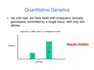
Identifying Genes Underlying Phenotypes • Linkage and quantitative trait locus (QTL) analysis • Need a pedigree with segregating traits • Linkage map with moderate number of markers • Very large regions of chromosomes represented by markers
Quantitative Trait Locus Mapping Parent 1 Parent 2 a b c a b c A B C A B C X HEIGHT F1 F1 A B C a b c bb Bb BB X GENOTYPE A B C a b c B b BB Bb BB bb bb BB Bb Bb BB A b c A B c A B c a B c a B c A b c a B c A b c a b c A b c A B C A B c A b c a B c a B c A b c a B c a B c
“Genetic architecture” of quantitative traits QTL studies can reveal the following facets of the genetic architecture of a quantitative trait: -Number of genes underlying the trait -The strength of effect of each gene -Additive vs. dominant effects of traits -Potential gene interactions among genes -Ultimately, “QTN” or the actual genes involved
Quantitative Trait Locus Analysis Step 1: Make a controlled cross to create a large family (or a collection of families) Parents should differ for phenotypes of interest Segregation of trait in the progeny Step 2: Create a genetic map Large number of markers phenotyped for all progeny Step 3: Measure phenotypes Need phenotypes with moderate to high heritability Step 4: Detect associations between markers and phenotype using a model Step 5: Identify underlying molecular mechanisms
Step 1: Construct Pedigree • Cross two individuals with contrasting characteristics • Create population with segregating traits • Ideally: inbred parents crossed to produce F1s, which are intercrossed to produce F2s • Recombinant Inbred Lines created by repeated intercrossing • Allows precise phenotyping, isolation of allelic effects Grisel 2000 Alchohol Research & Health 24:169
Step 2: Construct Genetic Map • Based on nonrandom association of alleles at different loci in pedigree • Calculate pairwise likelihood of linkage • Gives overview of structure of entire genome • Most efficient with anonymous markers: AFLP • Codominant markers much more informative: SSR
Step 3: Determine Phenotypes of Offspring • Phenotype must be segregating in pedigree • Must differentiate genotype and environment effects • How? • Works best with phenotypes with high heritability • Proportion of total phenotypic variance due to genetic effects • Why is this important? 0.1 0.5 0.9
Step 4: Detect Associations between Markers and Phenotypes • Single-marker associations are simplest • Simple ANOVA, correcting for multiple comparisons • Log likelihood ratio: LOD (Log10 of odds) • If QTL is between two markers, situation more complex • Recombination between QTL and markers (genotype doesn't predict phenotype) • 'Ghost' QTL due to adjacent QTL • Use interval mapping or composite interval mapping • Simultaneously consider pairs of loci across the genome
Step 5: Identify underlying molecular mechanisms QTL chromosome Genetic Marker QTG: Quantitative Trait Gene QTN: Quantitative Trait Nucleotide Adapted from Richard Mott, Wellcome Trust Center for Human Genetics
r A Q x a q a q a q QTL mapping: model for a single marker locus • Marker locus A, quantitative trait locus Q, recombine at rate r • Qq genotype has mean Qq • qq genotype has mean qq • Offspring • Aa has mean Aa=Qq (1-r) + qq r • aa has mean aa=Qq r + qq(1-r) • QTL effect = (Qq - qq )= (Aa-aa)/(1-2r) • Recombination rate confounded with QTL effect
r1 r2 A Q B a q b x a q b a q b QTL mapping: model for flanking marker loci • In simplest case, two markers A and B flank the QTL • Enough degrees of freedom to separately estimate QTL effect • "Interval mapping": estimate QTL effect in a sliding window along the marker map • Many approaches developed...
QTL map of in Douglas fir (bud opening date) Figure 2.—Seven QTL for terminal bud flush were detectedin the growth initiation experiment . QTL were found on six linkage groups (2, 3, 4, 5, 12, and 14) andwere detected in fiveof the six treatment combinations. Jermstad et al. (2003) Genetics, Vol. 165, 1489-1506
QTL Vary by Year, Site, and Population Loblolly pine QTL measured in different years at same site, in different sites, and with a different genetic background Stippled: not repeated across years % latewood wood-specific gravity Brown et al
Drawbacks of QTL mapping • Often results are difficult to reproduce, and vary by year, pedigree and location • Multiple experiments are needed to confirm results, but experiments are large undertakings (population size, genotyping, phenotyping) • Even if QTL localized to a few cM, this could correspond to 1000s of KB of DNA, containing many genes • As controlled crosses are used, only a fraction of natural variation surveyed • Biased towards detecting large effect QTL, as small effect QTL are not statistically significant
Association Genetics Methods for associating phenotypes with SNPs Effects of population structure Candidate gene approaches
Two approaches to association studies Population-based Cases (affected individuals) and unrelated population controls (unaffected individuals) collected from “one” population Effects of population structure can be incorporated Family-based Child-family trios and TDT design is the most common Robust to effects of population structure
Case – control association test • The simplest method • Compare SNP frequencies of affected vs. unaffected • Chi-square with one degree of freedom test C21 = (ad - bc)2N . (a+c)(b+d)(a+b)(c+d)
Knowler et al. (1988) collected data on 4920 Pima and Papago Native American populations in Southwestern United States High rate of Type II diabetes in these populations Found significant associations with Immunoglobin G marker (Gm) Does this indicate underlying mechanisms of disease? Case-Control Example: Diabetes
Case-control test for association (case=diabetic, control=not diabetic) = [(8x71)-(29x92)]2 (200) (100)(100)(37)(163) = 14.62 Gm Haplotype Question: Is the Gm haplotype associated with risk of Type 2 diabetes??? (1) Test for an association C21 = (ad - bc)2N . (a+c)(b+d)(a+b)(c+d) (2) Chi-square is significant. Therefore presence of GM haplotype seems to confer reduced occurence of diabetes. (Note the test is exactly analogous to calculating r2 between two loci).
Case-control test for association (continued) Question: Is the Gm haplotype actually associated with risk of Type 2 diabetes??? The real story: Stratify by American Indian heritage 0 = little or no indian heritage; 8 = complete indian heritage Conclusion: The Gm haplotype is NOT a risk factor for Type 2 diabetes, but is a marker of American Indian heritage
Family-Based Association: The Transmission Disequilibrium Test (TDT) Still an association test (like a case-control), but we study parents and offspring and we condition on the parental genotypes -this reduces effects of population stratification Given the genotypes of the parents, is there an allele that is transmitted more frequently to affected individuals? Only look at affected offspring with at least one heterozygous parent, and consider only family with affected progeny To do TDT, (1) we count the number of kids inheriting A or B across many families (trios) with affected kids AB AA Under the null hypothesis (H0) of no linkage, what proportion of alleles do we expect the heterozygous parent to transmit? (2) Statistically test whether this observed number is different from 50:50 AB or AA? (3) If NOT 50:50, then affected kids may be inheriting one allele preferentially over the other
AB AB AA AA Transmission Disequilibrium Test (TDT) (with known parental genotypes and 2 alleles at the locus) For each heterozygous parent in each family, we determine which allele is transmitted to the affected offspring and which is not. A B number=b A A number=c H0: Two alleles are transmitted equally (no linkage and no association) Ha: One of the alleles is preferentially transmitted (linkage and association) Test statistic is (b - c)2 ; c2 with 1 df b + c
1 2 1 1 1 2 1 1 1 2 1 1 10 families 15 families Transmission Disequilibrium Test (TDT) : Example For each heterozygous parent in each family, see which allele is transmitted to the affected offspring and which is not. TDT test b= , c= (b - c)2 = = , p-value = b + c
Methods for genetic association in natural populations • Standard general linear models (GLMs), usually with p values computed by permutation. • y = + mi + eij, where y is the trait value, is a general mean, mi is the genotype of the i-th SNP and eij is the residual. • Structured Association (Pritchard et al. 2000; Thornsberry 2001) and PCA Association (Price et al. 2006). • Controls for population structure by incorporating a Q matrix. This matrix is an n × p population structure incidence matrix where n is the number of individuals assayed and p is the number of populations defined. • Mixed Linear Models (MLMs; Yu et al. 2006). • They incorporate a Q matrix (fixed effect) but also a pairwise relatedness matrix (K matrix, a random effect), which account for within population structure.
Genetic association method depends upon population structure SA=structured association GC=genomic control GLM=general linear model TDT=transmission disequilibrium MLM=mixed linear model unknown Population structure GLM GC MLM SA GC MLM TDT GLM GC Familial relatedness Based on Yu & Buckler (2006) Current Opinion in Biotechnology
Pinus taeda L Pinus pinaster Ait. Fragmented range, significant population structure Continuous range, no clear population genetic structure TREESNIPS project (also P. sylvestris, Picea abies and oaks) ADEPT project
S3 microfibril angle 2o wall S2 S1 1o wall Genetic association with wood property traits in loblolly pine Phenotypic traits • Earlywood specific gravity (ewsg) • Latewood specific gravity (lwsg) • Percent latewood (lw) • Earlywood microfibril angle (ewmfa) • Lignin & cellulose content (lgn-cel) • Synthetic PCAs for different wood-age types González-Martínez et al. 2007 Genetics
Significant genetic association of cad gene with earlywood specific gravity and 4cl with % latewood 4cl cad
Genetic association method depends upon population structure SA=structured association GC=genomic control GLM=general linear model TDT=transmission disequilibrium MLM=mixed linear model unknown Population structure GLM GC MLM SA GC MLM TDT GLM GC Familial relatedness Based on Yu & Buckler (2006) Current Opinion in Biotechnology
Power considerations: structured populations Power % variation explained by QTN (Small association pop of ~100 accessions) Zhao et al. (2007) PLoS Genetics
Candidate Gene Associations vs. Whole Genome Scans Candidate Region QTL Candidate Gene Identification ABOVE:BELOW COARSE ROOT S3_1 163.4 S6_20 S13_31 171.3 T7_15 T2_31 178.2 S8_4 180.8 S8_28 182.1 O_30_A 184.2 T5_4 193.5 T3_17 198.1 T12_12 206.8 S5_29 210.6 P_2789_A 219.9 P_634_A S17_43 226.5 S17_33 230.3 S17_12 232.7 S4_19 243.1 S17_26 262.9 • If LD is high and haplotype blocks are conserved, entire genome can be efficiently scanned for associations with phenotypes • Simplest for case-control studies (e.g., disease, gender) • If LD is low, candidate genes are usually identified a priori, and a limited number are scanned for associations • Biased by existing knowledge • Use "Candidate Regions" from high LD populations, assess candidate genes in low LD populations I P_204_C 0.0 S8_32 8.8 P_2385_C P_2385_A 11.6 T4_10 12.1 S15_8 S5_37 13.8 T4_7 S6_12 15.5 S8_29 17.9 P_2786_A S12_18 20.4 T1_13 22.3 T7_4 23.5 T3_13 T3_36 24.1 S17_21 S15_16 T12_15 25.3 T2_30 26.5 S13_20 29.5 S1_20 36.5 T9_1 S1_19 43.2 50.5 S3_13 S1_24 52.9 S2_7 54.1 P_575_A 59.1 T12_22 60.6 S2_32 85.0 T7_9 95.7 S2_6 107.8 S13_16 T5_25 121.4 T5_12 124.3 T10_4 129.0 T1_26 T7_13 135.7 P_93_A 148.6 S4_20 150.2 S7_13 S7_12 152.8 T12_4 S4_24 T3_10 154.1 S6_4 P_2852_A 157.3
The “Candidate gene” approach • Candidate genes are selected by knowledge of how they influence similar traits in other organisms. • There is increasing evidence that some genes can control similar phenotypic traits even in distantly related species. • Easy to apply: lets see if this primer set works on this particular species!
Candidate gene definitions • Candidate genes are genes of known biological action involved with the development or physiology of the trait - Biological candidates • They may be structural genes or genes in a regulatory or biochemical pathway affecting trait expression • Positional candidates lie within the QTL region that affect the trait
Traditional candidate genes and traits • MHC related genes for studying disease and parasite resistance, and mate choice • Heat shock proteins (HSP) for temperature and stress tolerance • Growth hormone and its receptors for growth, size • Candidate genes also available for many ecologically relevant traits incl. morphology, color, foraging, learning and memory, social interactions, alternative mating strategies
Success story: Melanocortin-1 receptor gene • Coat colour variation in mice (Robbins et al. 1993) • Hair and skin color in humans (Valverde et al. 1995) • Feather coloration in chickens (Takeuchi et al. 1996) • Coat colour in pigs (Kijas et al. 1998) • Feather coloration in several bird species (Theron et al. 2001; Mundy et al. 2004) • Coat colour in several mammals such as horse, red fox and pocket mice (Mundy et al. 2004) • Skin color in lizards (Rosenblum et al. 2004). • Coat color of Kermode Bear(Ritland et al. 2001)
Melanocortin-1 receptor gene (MC1R) Mundy 2005
MC1R in pocket mouse Nachman et al. 2003
MC1R in pocket mouse: habitat differences Nachman et al. 2003
MC1R in lesser snow goose Mundy et al. 2004