GENOME MAPPING
GENOME MAPPING. Ms.ruchi yadav lecturer amity institute of biotechnology amity university lucknow (up). GENOME MAPPING. GENETIC MAPPING PHYSICAL MAPPING. GENOME MAPPING.

GENOME MAPPING
E N D
Presentation Transcript
GENOME MAPPING Ms.ruchiyadavlectureramity institute of biotechnologyamity universitylucknow(up)
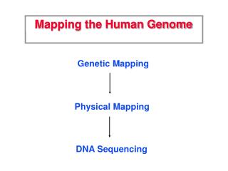
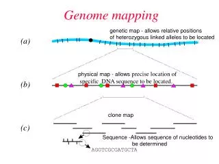
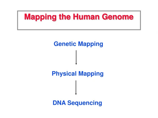
GENOME MAPPING GENETIC MAPPING PHYSICAL MAPPING
GENOME MAPPING • Genetic mapping is based on the use of genetic techniques to construct maps showing the positions of genes and other sequence features on a genome. • Genetic techniques include cross-breeding experiments or, • Case of humans, the examination of family histories (pedigrees). • Physical mapping uses molecular biology techniques to examine DNA molecules directly in order to construct maps showing the positions of sequence features, including genes.
DNA MARKERS FOR GENETIC MAPPING • Mapped features that are not genes are called DNA markers. As with gene markers, a DNA marker must have at least two alleles to be useful. There are three types of DNA sequence feature that satisfy this requirement: • Restriction fragment length polymorphisms (RFLPs) • Simple sequence length polymorphisms (SSLPs), and i) Minisatellites, also known as variable number of tandem repeats (VNTRs) in which the repeat unit is up to 25 bp in length; ii) Microsatellites or simple tandem repeats (STRs), whose repeats are shorter, usually dinucleotide or tetranucleotide units. • single nucleotide polymorphisms (SNPs).
Linkage analysis shows that the disease gene D lies between markers c and d.
RFLP • Distance between RFLP markers is also defined in recombination units or cM.
Amplified Fragment Length Polymorphism (AFLP) • AFLPs are differences in restriction fragment lengths caused by SNPs or INDELs that create or abolish restriction endonuclease recognition sites. • The AFLP technique is based on the selective PCR amplification of restriction fragments from a total digest of genomic DNA
RAPD (Random Amplified Polymorphic DNA) • RAPD markers are DNA fragments from PCR amplification of random segments of genomic DNA with single primer of arbitrary nucleotide sequence. • RAPD does not require any specific knowledge of the DNA sequence of the target organism • The identical 10-mer primers will or will not amplify a segment of DNA, depending on positions that are complementary to the primers' sequence.
Simple sequence length polymorphisms (SSLPs), • Unlike RFLPs, SSLPs can be multi-allelic as each SSLP can have a number of different length variants.
STRs • Advantages • Easy to detect via PCR • Lots of polymorphism • Co-dominant in nature • Disadvantage • Initial identification,DNA sequence information necessary
MAPPING TECHNIQUES • Linkage analysis is the basis of genetic mapping. • The offspring usually co-inherit either A with B or a with b, and, in this case, the law of independent assortment is not valid. • Thus to test for linkage between the genes for two traits, certain types of matings are examined and observe whether or not the pattern of the combinations of traits exhibited by the offspring follows the law of independent assortment. • If not, the gene pairs for those traits must be linked, that is they must be on the same chromosome pair.
What types of matings can reveal that the genes for two traits are linked? • Only matings involving an individual who is heterozygous for both traits (genotype AaBb) reveal deviations from independent assortment and thus reveal linkage. • Moreover, the most obvious deviations occur in the test cross, a mating between a double heterozygote and a doubly recessive homozygote (genotype aabb). • Individuals with the genotype AaBb manifest both dominant phenotypes; those with the genotype aabb manifest both recessive phenotypes.
How do we estimate, from the offspring of a single family, the likelihood that two gene pairs are linked? • Recombination fraction • LOD score • Haldane mapping function
Recombination Frequency • Recombination fraction is a measure of the distance between two loci. • Two loci that show 1% recombination are defined as being 1 centimorgan (cM) apart on a genetic map. • 1 map unit = 1 cM (centimorgan) • Two genes that undergo independent assortment have recombination frequency of 50 percent and are located on nonhomologous chromosomes or far apart on the same chromosome = unlinked • Genes with recombination frequencies less than 50 percent are on the same chromosome = linked
Calculation of Recombination Frequency • The percentage of recombinant progeny produced in a cross is called the recombination frequency, which is calculated as follows:
LOD SCORE • The LOD score is calculated as follows: • LOD = Z = Log10 probability of birth sequence with a given linkage probability of birth sequence with no linkage • By convention, a LOD score greater than 3.0 is considered evidence for linkage. • On the other hand, a LOD score less than -2.0 is considered evidence to exclude linkage.
LOD Score Analysis • The likelihood ratio as defined by :- L(pedigree| = x) L(pedigree | = 0.50) • where represents the recombination fraction and where 0 x 0.49. • L.R. = • TheLOD score (z) is the log10 (L.R.)
Method to evaluate the statistical significance of results. • Maximum-likelihood analysis, which estimates the “most likely” value of the recombination fraction Ø as well as the odds in favour of linkage versus nonlinkage. • Given by Conditional probability L(data 1 Ø), which is the likelihood of obtaining the data if the genes are linked and have a recombination fraction of Ø. • Likelihood of obtaining one recombinant and seven nonrecombinants when the recombination fraction is Ø is proportional to Ø1(1–Ø)7, Where:Ø is, by definition, the probability of obtaining a recombinant , (I – Ø) is the probability of obtaining a nonrecombinant.
Mappingfunction • The genetic distance between locus A and locus B is defined as the average number of crossovers occurring in the interval AB. • Mapping function is use to translate recombination fractions into genetic distances. • In 1919 the British geneticist J, B. S. Haldane proposed such Mapping function • Haldane defined the genetic distance, x, between two loci as the average number of crossovers per meiosis in the interval between the two loci.
What is Haldane ’s mapping function ? • Assumptions: crossovers occurred at random along the chromosome and that the probability of a crossover at one position along the chromosome was independent of the probability of a crossover at another position. • Using these assumptions, he derived the following relationship between • Ø, the recombination fraction and • x ,the genetic distance (in morgans): Ø=1/2(1-e-2x) or equivalently, X=-1/2ln(1-2Ø)
Genetic distance between two loci increases, the recombination fraction approaches a limiting value of 0.5. • Cytological observations of meiosis indicate that the average number of crossovers undergone by the chromosome pairs of a germ-line cell during meiosis is 33. • Therefore, the average genetic length of a human chromosome is about 1.4 morgans, or about140 centimorgans.
LIMITATIONS • A map generated by genetic techniques is rarely sufficient for directing the sequencing phase of a genome project. This is for two reasons: • The resolution of a genetic map depends on the number of crossovers that have been scored . • Genes that are several tens of kb apart may appear at the same position on the genetic map. • Genetic maps have limited accuracy . • Presence of recombination hotspots means that crossovers are more likely to occur at some points rather than at others. • physical mapping techniques has been developed to address this problem.
Physical mapping • Actual physical distances • Units in base-pairs • Contigs of large DNA fragments • Large insert DNA libraries (BACs, PACs, etc) • Restriction fragment fingerprinting • Minimum tiling set to cover entire genome • Correlation of genetic and physical maps • Genetic marker screening • EST screening • BAC-end sequencing • FISH
PHYSICAL MAPPING • Restriction mapping, which locates the relative positions on a DNA molecule of the recognition sequences for restriction endonucleases; • Fluorescent in situ hybridization (FISH), in which marker locations are mapped by hybridizing a probe containing the marker to intact chromosomes; • Sequence tagged site (STS) mapping, in which the positions of short sequences are mapped by PCR and/or hybridization analysis of genome fragments.
Restriction mapping • partial restriction
Physical maps • Physical maps can be generated by aligning the restriction maps of specific pieces of cloned genomic DNA (for instance, in YAC or BAC vectors) along the chromosomes. • These maps are extremely useful for the purpose of map-based gene cloning.
Fluorescent in situ hybridization (FISH) • FISH enables the position of a marker on a chromosome or extended DNA molecule to be directly visualized • In FISH, the marker is a DNA sequence that is visualized by hybridization with a fluorescent probe. • In situ hybridization intact chromosome is examined by probing it with a labeled DNA molecule.
In situ hybridization with radioactive or fluorescent probes • The position on the chromosome at which hybridization occurs provides information about the map location of the DNA sequence used as the probe • DNA in the chromosome is made single stranded (‘denatured’). • The standard method for denaturing chromosomal DNA without destroying the morphology of the chromosome is to dry the preparation onto a glass microscope slide and then treat with formamide.
Can distinguish chromosomes by “painting” – using DNA hybridization + fluorescent probes – during mitosis