Bump Mapping
Bump Mapping. Mohan Sridharan Based on slides created by Edward Angel. Introduction. Mapping methods: Texture mapping. Environmental (reflection) mapping: Variant of texture mapping. Bump mapping: Solves flatness problem of texture mapping. Examples. Modeling an Orange.

Bump Mapping
E N D
Presentation Transcript
Bump Mapping Mohan Sridharan Based on slides created by Edward Angel CS4395: Computer Graphics
Introduction • Mapping methods: • Texture mapping. • Environmental (reflection) mapping: • Variant of texture mapping. • Bump mapping: • Solves flatness problem of texture mapping. CS4395: Computer Graphics
Examples CS4395: Computer Graphics
Modeling an Orange • Consider modeling an orange. • Texture map a photo of an orange onto a surface: • Captures dimples. • Will not be correct if we move viewer or light. • We have shades of dimples rather than their correct orientation. • We need to perturb normal across surface of object and compute a new color at each interior point. CS4395: Computer Graphics
Bump Mapping (Blinn) • Consider a smooth surface: n p CS4395: Computer Graphics
Rougher Version n’ p’ p CS4395: Computer Graphics
Equations p(u,v) = [x(u,v), y(u,v), z(u,v)]T pu=[ ∂x/ ∂u, ∂y/ ∂u, ∂z/ ∂u]T pv=[ ∂x/ ∂v, ∂y/ ∂v, ∂z/ ∂v]T n = (pupv ) / |pupv| CS4395: Computer Graphics
Tangent Plane pv n pu CS4395: Computer Graphics
Displacement Function p’ = p + d(u,v) n d(u,v) is the bump or displacement function. |d(u,v)| << 1 CS4395: Computer Graphics
Perturbed Normal n’ = p’up’v p’u=pu + (∂d/∂u)n + d(u,v)nu p’v=pv + (∂d/∂v)n + d(u,v)nv If d is small, we can neglect last term. CS4395: Computer Graphics
Approximating the Normal n’ = p’up’v ≈ n + (∂d/∂u)n pv + (∂d/∂v)n pu The vectors n pv and n pu lie in the tangent plane. Hence the normal is displaced in the tangent plane . Must pre-compute the arrays ∂d/ ∂u and ∂d/ ∂v Finally, we perturb the normal during shading. CS4395: Computer Graphics
Image Processing • Suppose that we start with a function d(u,v). • We can sample it to form an array D=[dij]. • Then ∂d/ ∂u ≈ dij – di-1,j and ∂d/ ∂v ≈ dij – di,j-1 • Embossing: multi-pass approach using accumulation buffer. CS4395: Computer Graphics
How to do this? • The problem is that we want to apply the perturbation at all points on the surface. • Cannot solve by vertex lighting (unless polygons are very small). • Really want to apply to every fragment. Can not do that in fixed function pipeline. • But can do with a fragment program – later CS4395: Computer Graphics