
Outline
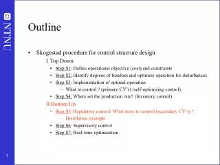
Outline. Skogestad procedure for control structure design I Top Down Step S1 : Define operational objective (cost) and constraints Step S2: Identify degrees of freedom and optimize operation for disturbances Step S3 : Implementation of optimal operation

Outline
E N D
Presentation Transcript
Outline • Skogestad procedure for control structure design I Top Down • Step S1: Define operational objective (cost) and constraints • Step S2: Identify degrees of freedom and optimize operation for disturbances • Step S3: Implementation of optimal operation • What to control ? (primary CV’s) (self-optimizing control) • Step S4: Where set the production rate? (Inventory control) II Bottom Up • Step S5: Regulatory control: What more to control (secondary CV’s) ? • Distillation example • Step S6: Supervisory control • Step S7: Real-time optimization
II. Bottom-up • Determine secondary controlled variables and structure (configuration) of control system (pairing) • A good control configuration is insensitive to parameter changes
y1 = c y2 = ? Regulatory control layer • Purpose: “Stabilize” the plant using a simple control configuration (usually: local SISO PID controllers + simple cascades) • Enable manual operation (by operators) • Step S5: Regulatory / stabilizing control (PID layer) (a) What more to control (CV2=y2; local CVs)? (Decision 2) (b) Pairing of inputs u2 and outputs y2 (Decision 4)
Optimizer (RTO) Optimally constant valves CV1s Always active constraints y1=CV1 Supervisory controller (MPC) CV2s y2=CV2 Regulatory controller (PID) H H2 Physical inputs (valves) d y PROCESS Stabilized process ny u2 Degrees of freedom for optimization (usually steady-state DOFs), MVopt = CV1s Degrees of freedom for supervisory control, MV1=CV2s + unused valves Physical degrees of freedom for stabilizing control, MV2 = valves (dynamic process inputs)
Objectives regulatory control layer • Allow for manual operation • Simple decentralized (local) PID controllers that can be tuned on-line • Take care of “fast” control • Track setpoint changes from the layer above • Local disturbance rejection • Stabilization (mathematical sense) • Avoid “drift” (due to disturbances) so system stays in “linear region” • “stabilization” (practical sense) • Allow for “slow” control in layer above (supervisory control) • Make control problem easy as seen from layer above
Details Step 5 (Structure regulatory control layer) (a) What to control? • Control CV2s (y2) that “stabilizes the plant” (stops drifting) • Select y2 which is easy to control (favorable dynamics) • Favor reliable measurements y2 2. In addition, active constraints (CV1) that require tight control (small backoff) may be assigned to the regulatory layer.* • *Comment: usually not necessary with tight control of unconstrained CVs because optimum is usually relatively flat
“Control CV2s that “stabilizes the plant” (stops drifting)” A. “Mathematical stabilization” (e.g. reactor): • Unstable mode is “quickly” detected (state observability) in the measurement (y2) and is easily affected (state controllability) by the input (u2). • Tool for selecting input/output: Pole vectors • y2: Want large element in output pole vector: Instability easily detected relative to noise • u2: Want large element in input pole vector: Small input usage required for stabilization B. “Practical extended stabilization” (avoid “drift” due to disturbance sensitivity): • Intuitive: y2 located close to important disturbance • Maximum gain rule:Controllable range for y2 is large compared to sum of optimal variation and measurement+control error • More exact tool: Partial control analysis
“Control CV2s that stabilizes the plant (stops drifting)”In practice, control: • Levels (inventory liquid) • Pressures (inventory gas/vapor) (note: some pressures may be left floating) • Inventories of components that may accumulate/deplete inside plant • E.g., amount of amine/water (deplete) in recycle loop in CO2 capture plant • E.g., amount of butanol (accumulates) in methanol-water distillation column • E.g., amount of inert N2 (accumulates) in ammonia reactor recycle • Reactor temperature • Distillation column profile (one temperature inside column) • Stripper/absorber profile does not generally need to be stabilized
2. “y2 is easy to control” (controllability) • Steady state: Want large gain (from u2 to y2) • Dynamics: Want small effective delay(from u2 to y2) • “effective delay” includes • inverse response (RHP-zeros) • + high-order lags Main rule: y2 is easy to measure and located close to available manipulated variable u2 (“pairing”)
What should we control (y2)? • Avoid closing too many loops because it increases complexity
Details Step 5b…. (b) Identify pairings = Identify MVs (u2) to be used to control CV2, taking into account • Want “local consistency” for the inventory control • Implies radiating inventory control around given flow • Avoid selecting as MVs in the regulatory layer (u2), variables that may optimally saturate at steady-state (active constraint on some region), because this would require either • reassigning the regulatory loop (complication penalty), or • requiring back-off for the MV variable (economic penalty) • Avoid variables u2 where (frequent) changes are undesirable, for example, because they disturb other parts of the process. • Want tight control of important active constraints (to avoid back-off) • General rule: ”pair close” (see next slide) Comments: • Preferably, the regulatory layer should be independent of the economics (operating regions of active constraints) - without the need to reassigning loops depending on disturbances, price changes, etc. • The total number of theoretical pairing options is very large, but in practice, by following the above rules, the number is usually quite small (in some cases, there may be no feasible solution, so, for example, the radiating rule must be broken)
Step 5b…. Further Rules for pairing of variables Main rule: “Pair close” • The response (from input to output) should be fast, large and in one direction. Avoid dead time and inverse responses! • The input (MV) should preferably effect only one output (to avoid interaction between the loops) • Try to avoid input saturation (valve fully open or closed) in “basic” control loops for level and pressure • The measurement of the output y should be fast and accurate. It should be located close to the input (MV) and to important disturbances. • Use extra measurements y’ and cascade control if this is not satisfied • The system should be simple • Avoid too many feedforward and cascade loops • “Obvious” loops (for example, for level and pressure) should be closed first before you spend to much time on deriving process models, RGA-analysis, etc.
Why simplified configurations?Why control layers?Why not one “big” multivariable controller? • Fundamental: Save on modelling effort • Other: • easy to understand • easy to tune and retune • insensitive to model uncertainty • possible to design for failure tolerance • fewer links • reduced computation load
Closing inner loops (cascade control):Use of (extra) measurements (y2) as (extra) CVs Primary CV y1 y2s K u2 G y2 Secondary CV (control for dynamic reasons) Key decision: Choice of y2 (controlled variable) Also important: Choice of u2 (“pairing”)
y1 y2s K u2 G y2 Original DOF New DOF Degrees of freedom unchanged • No degrees of freedom lost by control of secondary (local) variables as setpoints become y2s replace inputs u2 as new degrees of freedom Cascade control:
Hierarchical/cascade control: Time scale separation • With a “reasonable” time scale separation between the layers (typically by a factor 5 or more in terms of closed-loop response time) we have the following advantages: • The stability and performance of the lower (faster) layer (involving y2) is not much influenced by the presence of the upper (slow) layers (involving y1) Reason: The frequency of the “disturbance” from the upper layer is well inside the bandwidth of the lower layers • With the lower (faster) layer in place, the stability and performance of the upper (slower) layers do not depend much on the specific controller settings used in the lower layers Reason: The lower layers only effect frequencies outside the bandwidth of the upper layers
Cascade control distillation ys With flow loop + T-loop in top y XC Ts T TC Ls L FC z XC
Summary step 5: Rules for selecting y2 (and u2) Selection of y2 • Control of y2 “stabilizes” the plant • Control variables that “drift” • The (scaled) gain for y2 should be large • Measurement of y2 should be simple and reliable • For example, temperature or pressure • y2 should have good controllability • small effective delay • favorable dynamics for control • y2 should be located “close” to a manipulated input (u2) Selection of u2 (to be paired with y2): • Avoid using inputs u2 that may saturate (at steady state) • When u2 saturates we loose control of the associated y2. • Avoid variables u2 where (frequent) changes are undesirable • For example, they may disturb other parts of the process. • The effective delay from u2 to y2 should be small (“pair close”!)
QUIZ: What are the benefits of adding a flow controller (inner cascade)? qs Extra measurement y2 = q q z • Counteracts nonlinearity in valve, f(z) • With fast flow control we can assume q = qs • Eliminates effect of disturbances in p1 and p2
Example regulatory control: Distillation • Assume given feed • 5 dynamic DOFs (L,V,D,B,VT) • Overall objective: • Control compositions (xD and xB) • “Obvious” stabilizing loops: • Condenser level (M1) • Reboiler level (M2) • Pressure E.A. Wolff and S. Skogestad, ``Temperature cascade control of distillation columns'', Ind.Eng.Chem.Res., 35, 475-484, 1996.
The dos and don’ts of distillation column control Sigurd Skogestad Norwegian University of Science and Technology – NTNU N-7491 Trondheim, Norway From: Plenary lecture Distillation’06, London, 05 Sep 2006 Will mainly consider (indirect) composition control
Studied in hundreds of research and industrial papers over the last 60 years
L Ts TC TC V Issues distillation control • The “configuration” problem (level and pressure control) • Which are the two remaining degrees of freedom? • e.g. LV-, DV-, DB- and L/D V/B-configurations • The temperature control problem • Which temperature (if any) should be controlled? • Composition control problem • Control two, one or no compositions?
Objectives of this work • Apply general plantwide control procedure (Skogestad, 2004) to distillation • From this derive (if possible) simple recommendations for distillation control • Is the latter possible? Luyben (2006) has his doubts: • “There are many different types of distillation columns and many different types of control structures. The selection of the ``best'' control structure is not as simple as some papers* claim. Factors that influence the selection include volatilities, product purities, reflux ratio, column pressure, cost of energy, column size and composition of the feed”+ prices products * He may be referring to my work...
2. General procedure plantwide control Step I. “Top-down” steady-state approach to identify primary controlled variables (y1) • Active constraints • Self-optimizing control Step II. Bottom-up identification of regulatory (“stabilizing”) control layer. • Identify secondary controlled variables (y2) y1s Control of primary variables: compositions (MPC) y2s “Stabilizing” control: p, levels, T (PID)
Selection of primary CVs (y1) 3. Primary controlled variables distillation (y1) cost energy (heating+ cooling) • Cost to be minimized (economics) J = - P where P= pD D + pB B – pF F – pV V • Constraints Purity D: For example xD, impurity· max Purity B: For example, xB, impurity· max Flow constraints: 0 · D, B, L etc. · max Column capacity (flooding): V · Vmax, etc. value products cost feed
Selection of primary CVs (y1) methanol + water valuable product methanol + max. 0.5% water cheap product (byproduct) water + max. 0.1% methanol Expected active constraints distillation • Valueable product: Purity spec. always active • Reason: Amount of valuable product (D or B) should always be maximized • Avoid product “give-away” (“Sell water as methanol”) • Also saves energy • Control implications: ALWAYS Control valueable purity at spec.
Selection of primary CVs (y1) methanol + water valuable product methanol + max. 0.5% water cheap product (byproduct) water + max. 0.1% methanol Cheap product • Over-fractionate cheap product? Trade-off: • Yes, increased recovery of valuable product (less loss) • No, costs energy • Control implications cheap product: • Energy expensive: Purity spec. active → Control purity at spec. • Energy “cheap”: Overpurify • Unconstrained optimum given by trade-off between energy and recovery. In this case it is likely that composition is self-optimizing variable → Possibly control purity at optimum value (overpurify) (b) Constrained optimum given by column reaching capacity constraint → Control active capacity constraint (e.g. V=Vmax) • Methanol + water example: Since methanol loss anyhow is low (0.1% of water), there is not much to gain by overpurifying. Nevertheless, with energy very cheap, it is probably optimal to operate at V=Vmax.
Selection of primary CVs (y1) Conclusion primary controlled variables • Product purities are very often the primary controlled variables (y1) for distillation columns • Assume in the following “two-point” composition control: y1 = xD, xB (impurity key component)
4. Stabilizing control distillationSecondary controlled variables (y2) • 5 dynamic degrees of freedom with given feed: L, V, D, B, VT • To “stabilize”: Control levels and pressure: y2 = MD, MB, p • Choice of input u2 (to be paired with y2): • VT is usually used to control p • Levels (MD and MB): Many possible configurations • Additional y2: Temperature is usually controlled to “stabilize” composition profile:
Configurations 5. Control “configurations” (pairing u2-y2 for level control) • “XY-configuration” X: remaining input in top after controlling top level (MD): X= L (reflux), D, L/D,… Y: remaining input in bottom after controlling MB: Y = V (boilup, energy input), B, V/B, ...
Configurations LC Top of Column cooling VT LS “Standard” : LY-configuration (“energy balance”) L+D D L Set manually or from upper-layer controller (temperature or composition) Set manually or from upper-layer controller VT DS LC “Reversed”: DY-configuration (“material balance”) D L
Configurations Top of Column VT LC D L D Ls Set manually or from upper-layer controller (L/D)s x Similar in bottom... XV, XB, X V/B
LV-configuration (most common) • “LV-configuration”: • D and B for levels (“local consistent”) • L and V remain as degrees of freedom • after level loops are closed • Other possibilities: • DB, L/D V/B, etc….
Configurations How do the configurations differ? • Has been a lot of discussion in the literature (Shinskey, Buckley, Skogestad, Luyben, etc.). • Probably over-emphasized • Level control by itself (emphasized by Buckley et al., 1985) • Interaction of level control with composition control • Related to “local consistency” (Do not want inventory control to depend on composition loops being closed) • “Self-regulation” in terms of disturbance rejection (emphasized by Skogestad and Morari, 1987) • Remaining two-point composition control problem (steady-state RGA - emphasized by Shinskey, 1984) BUT: These comparisons are mostly without temperature control…..
BUT: To avoid strong sensitivity to disturbances: Temperature profile must also be “stabilized” D feedback using e.g. D,L,V or B LIGHT TC F HEAVY B Even with the level and pressure loops closed the column is practically unstable - either close to integrating or even truly unstable ( e.g. with mass reflux: Jacobsen and Skogestad, 1991) • To stabilize the column we must use feedback (feedforward will give drift) • Simplest: “Profile feedback” using sensitive temperature
Stabilizing the column profile • Should close one “fast” loop (usually temperature) in order to “stabilize” the column profile • Makes column behave more linearly • Strongly reduces disturbance sensitivity • Keeps disturbances within column • Reduces the need for level control • Makes it possible to have good dual composition control • P-control usually OK (no integral action) • Similar to control of liquid level
• Which fast loop should be closed (“pairing”)? Btm Btm . loop . loop – Which end? Close loop in end with “most important” using V using V product LV LV LV – Which output (temperature)? Choose “sensitive” stage – Which input (flow)? Want fast control “pair close” ) T T T s s s TC TC TC • “Use same end” (reduces interactions for composition control): – Use V (or indirect by B) for temperature control in bottom section – Use L (or indirect by D) for temperature control in top section • Dynamics – L: Some delay for liquid to go down the column – V: Vapor flow moves quickly up the column, but may take some time before it starts changing (heat transfer dynamics) Top loop Top loop • In general, for stabilizing loops: Avoid using an input (flow) using L using L that can saturate TC TC TS – Do not use boilup (V) if column is close to max. capacity Stabilizing the column profile
TC Bonus 1 of temp. control: Indirect level control Disturbance in V, qF: Detected by TC and counteracted by L -> Smaller changes in D required to keep Md constant!
Bonus 2 of temp. control: Less interactive Setpoint T: New “handle” instead of L Ts TC
Less interactive: Closed-loop response with decentralized PID-composition control Interactions much smaller with “stabilizing” temperature loop closed … and also disturbance sensitivity is expected smaller %
Integral action in inner temperature loop has little effect %
Note: No need to close two inner temperature loops % Would be even better with V/F
Would be even better with V/F: Ts TC F (V/F)s x V
x (L/F)s Ts TC A “winner”: L/F-T-conguration Only caution: V should not saturate
TC Temperature control: Which stage?
Which temperature?Rule: Maximize the scaled gain • Scalar case. Minimum singular value = gain |G| • Maximize scaled gain: |G| = |G0| / span • |G0|: gain from independent variable (u) to candidate controlled variable (c) • span (of c) = variation (of c) = optimal variation in c + control error for c
Binary distillation: Unscaled steady-state gain G0 = ΔT/ΔL for small change in L T / L BTM TOP
Procedure scaling • Nominal simulation • Unscaled gains (“steady-state sensitivity”) • Make small change in input (L) with the other inputs (V) constant. • Find gain = Ti/ L • Do the same for change in V • Obtain scalings (“optimal variation for various disturbances”) • Find Ti,opt for the following disturbances • F (from 1 to 1.2) yoptf • zF from 0.5 to 0.6 yoptz • “Optimal” variation yopt to disturbances: Keep constant xD and xB by changing both L and V (disturbance in F has no effect in this case, so yoptf=0) • Control (implementation) error. Assume=0.5 K on all stages • Find • scaled-gain = gain/span • where span = abs(yoptf)+abs(yoptz)+0.5 • “Maximize gain rule”: Prefer stage where scaled-gain is large


