Query Processing and Optimization: Techniques & Algorithms
Understand query optimization strategies, translate SQL queries into relational algebra, implement select and join operations using various algorithms, and explore factors affecting join performance.

Query Processing and Optimization: Techniques & Algorithms
E N D
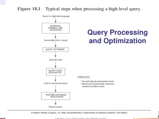
Presentation Transcript
Query Processing and Optimization • Query optimization: the process of choosing a suitable execution strategy for processing a query. • Two internal representations of a query • Query Tree • Query Graph • Query block: the basic unit that can be translated into the algebraic operators and optimized. A query block contains a single SELECT-FROM-WHERE expression, as well as GROUP BY and HAVING clause if these are part of the block. • Nested queries within a query are identified as separate query blocks.
Translating SQL Queries into Relational Algebra SELECT LNAME, FNAME FROM EMPLOYEE WHERE SALARY > ( SELECT MAX (SALARY) FROM EMPLOYEE WHERE DNO = 5); SELECT LNAME, FNAME FROM EMPLOYEE WHERE SALARY > C SELECT MAX (SALARY) FROM EMPLOYEE WHERE DNO = 5 πLNAME, FNAME(σSALARY>C(EMPLOYEE)) ℱMAX SALARY(σDNO=5 (EMPLOYEE))
Algorithms for SELECT and JOIN Operations (1) Implementing the SELECT Operation: • Examples: (OP1): sSSN='123456789' (EMPLOYEE) (OP2): sDNUMBER>5(DEPARTMENT) (OP3): sDNO=5(EMPLOYEE) (OP4): sDNO=5 AND SALARY>30000 AND SEX=F(EMPLOYEE) (OP5): sESSN=123456789 AND PNO=10(WORKS_ON)
Algorithms for SELECT and JOIN Operations (2) Implementing the SELECT Operation (cont.): • S1. Linear search (brute force): Retrieve every record in the file, and test whether its attribute values satisfy the selection condition. • S2. Binary search: If the selection condition involves an equality comparison on a key attribute on which the file is ordered, binary search (which is more efficient than linear search) can be used. (See OP1). • S3. Using a primary index or hash key to retrieve a single record: If the selection condition involves an equality comparison on a key attribute with a primary index (or a hash key), use the primary index (or the hash key) to retrieve the record. • S4. Using a primary index to retrieve multiple records: If the comparison condition is >, ≥, <, or ≤ on a key field with a primary index, use the index to find the record satisfying the condition • S5. Using a clustering index to retrieve multiple records: If the selection condition involves an equality comparison on a non-key attribute with a clustering index • S6.Using a secondary (B+-tree) index: On an equality comparison, this search method can be used to retrieve a single record if the indexing field has unique values (is a key) or to retrieve multiple records if the indexing field is not a key. In addition, it can be used to retrieve records on conditions involving >,>=, <, or <=. (FOR RANGE QUERIES)
Algorithms for SELECT and JOIN Operations (3) Implementing the JOIN Operation: • Join (EQUIJOIN, NATURAL JOIN) • two–way join: a join on two files e.g. R A=B S • multi-way joins: joins involving more than two files. e.g. R A=B S C=D T • Examples (OP6): EMPLOYEE DNO=DNUMBER DEPARTMENT (OP7): DEPARTMENT MGRSSN=SSN EMPLOYEE
Algorithms for SELECT and JOIN Operations (4) Implementing the JOIN Operation (cont.): Methods for implementing joins: • J1. Nested-loop join (brute force): For each record t in R (outer loop), retrieve every record s from S (inner loop) and test whether the two records satisfy the join condition t[A] = s[B]. • J2. Single-loop join (Using an access structure to retrieve the matching records): If an index (or hash key) exists for one of the two join attributes — say, B of S — retrieve each record t in R, one at a time, and then use the access structure to retrieve directly all matching records s from S that satisfy s[B] = t[A].
Algorithms for SELECT and JOIN Operations (5) Implementing the JOIN Operation (cont.): Methods for implementing joins: • J3. Sort-merge join: If the records of R and S are physically sorted (ordered) by value of the join attributes A and B, respectively, we can implement the join in the most efficient way possible. Both files are scanned in order of the join attributes, matching the records that have the same values for A and B. In this method, the records of each file are scanned only once each for matching with the other file—unless both A and B are non-key attributes, in which case the method needs to be modified slightly. • J4. Hash-join: The records of files R and S are both hashed to the same hash file, using the same hashing function on the join attributes A of R and B of S as hash keys. A single pass through the file with fewer records (say, R) hashes its records to the hash file buckets. A single pass through the other file (S) then hashes each of its records to the appropriate bucket, where the record is combined with all matching records from R.
Algorithms for SELECT and JOIN Operations (6) Implementing the JOIN Operation (cont.): • Factors affecting JOIN performance • Available buffer space • Join selection factor • Choice of inner VS outer relation
Using Heuristics in Query Optimization (1) • Example: For every project located in ‘Stafford’, retrieve the project number, the controlling department number and the department manager’s last name, address and birthdate. Relation algebra: PNUMBER, DNUM, LNAME, ADDRESS, BDATE (((PLOCATION=‘STAFFORD’(PROJECT)) DNUM=DNUMBER (DEPARTMENT)) MGRSSN=SSN (EMPLOYEE)) SQL query: Q2: SELECT P.NUMBER,P.DNUM,E.LNAME, E.ADDRESS, E.BDATE FROM PROJECT AS P,DEPARTMENT AS D, EMPLOYEE AS E WHERE P.DNUM=D.DNUMBER AND D.MGRSSN=E.SSN AND P.PLOCATION=‘STAFFORD’;
Using Heuristics in Query Optimization (3) Heuristic Optimization of Query Trees: • The same query could correspond to many different relational algebra expressions — and hence many different query trees. • The task of heuristic optimization of query trees is to find a final query tree that is efficient to execute. • Example: Q: SELECT LNAME FROM EMPLOYEE, WORKS_ON, PROJECT WHERE PNAME = ‘AQUARIUS’ AND PNMUBER=PNO AND ESSN=SSN AND BDATE > ‘1957-12-31’;
8. Using Selectivity and Cost Estimates in Query Optimization (1) • Cost-based query optimization: Estimate and compare the costs of executing a query using different execution strategies and choose the strategy with the lowest cost estimate. (Compare to heuristic query optimization) • Issues • Cost function • Number of execution strategies to be considered
Using Selectivity and Cost Estimates in Query Optimization (2) • Cost Components for Query Execution • Access cost to secondary storage • Storage cost • Computation cost • Memory usage cost • Communication cost Note: Different database systems may focus on different cost components.
Using Selectivity and Cost Estimates in Query Optimization (3) • Catalog Information Used in Cost Functions • Information about the size of a file • number of records (tuples) (r), • record size (R), • number of blocks (b) • blocking factor (bfr) • Information about indexes and indexing attributes of a file • Number of levels (x) of each multilevel index • Number of first-level index blocks (bI1) • Number of distinct values (d) of an attribute • Selectivity (sl) of an attribute • Selection cardinality (s) of an attribute. (s = sl * r)
Using Selectivity and Cost Estimates in Query Optimization (4) Examples of Cost Functions for SELECT • S1. Linear search (brute force) approach CS1a = b; For an equality condition on a key, CS1a = (b/2) if the record is found; otherwise CS1a = b. • S2. Binary search: CS2 = log2b + ┌(s/bfr) ┐–1 For an equality condition on a unique (key) attribute, CS2 =log2b • S3. Using a primary index (S3a) or hash key (S3b) to retrieve a single record CS3a = x + 1; CS3b = 1 for static or linear hashing; CS3b = 1 for extendible hashing;
Using Selectivity and Cost Estimates in Query Optimization (5) Examples of Cost Functions for SELECT (cont.) • S4. Using an ordering index to retrieve multiple records: For the comparison condition on a key field with an ordering index, CS4 = x + (b/2) • S5. Using a clustering index to retrieve multiple records: CS5 = x + ┌ (s/bfr) ┐ • S6. Using a secondary (B+-tree) index: For an equality comparison, CS6a = x + s; For an comparison condition such as >, <, >=, or <=, CS6a = x + (bI1/2) + (r/2)
Using Selectivity and Cost Estimates in Query Optimization (6) Examples of Cost Functions for JOIN • Join selectivity (js) js = | (R C S) | / | R x S | = | (R C S) | / (|R| * |S |) If condition C does not exist, js = 1; If no tuples from the relations satisfy condition C, js = 0; Usually, 0 <= js <= 1; • Size of the result file after join operation | (R C S) | = js * |R| * |S |
Using Selectivity and Cost Estimates in Query Optimization (7) Examples of Cost Functions for JOIN (cont.) • J1. Nested-loop join: CJ1 = bR + (bR*bS) + ((js* |R|* |S|)/bfrRS) (Use R for outer loop) • J2. Single-loop join (using an access structure to retrieve the matching record(s)) If an index exists for the join attribute B of S with index levels xB,we can retrieve each record s in R and then use the index to retrieve all the matching records t from S that satisfy t[B] = s[A]. The cost depends on the type of index.
Using Selectivity and Cost Estimates in Query Optimization (8) Examples of Cost Functions for JOIN (cont.) • J2. Single-loop join (cont.) For a secondary index, CJ2a = bR + (|R| * (xB + sB)) + ((js* |R|* |S|)/bfrRS); For a clustering index, CJ2b = bR + (|R| * (xB + (sB/bfrB))) + ((js* |R|* |S|)/bfrRS); For a primary index, CJ2c = bR + (|R| * (xB + 1)) + ((js* |R|* |S|)/bfrRS); If a hash key exists for one of the two join attributes — B of S CJ2d = bR + (|R| * h) + ((js* |R|* |S|)/bfrRS); • J3. Sort-merge join: CJ3a = CS + bR + bS + ((js* |R|* |S|)/bfrRS); (CS: Cost for sorting files)
9. Overview of Query Optimization in Oracle Oracle DBMS V8 • Rule-based query optimization: the optimizer chooses execution plans based on heuristically ranked operations. (Currently it is being phased out) • Cost-based query optimization: the optimizer examines alternative access paths and operator algorithms and chooses the execution plan with lowest estimate cost. The query cost is calculated based on the estimated usage of resources such as I/O, CPU and memory needed. • Application developers could specify hints to the ORACLE query optimizer. The idea is that an application developer might know more information about the data.
10. Semantic Query Optimization • Semantic Query Optimization: Uses constraints specified on the database schema in order to modify one query into another query that is more efficient to execute. • Consider the following SQL query, SELECT E.LNAME, M.LNAME FROM EMPLOYEE E M WHERE E.SUPERSSN=M.SSN AND E.SALARY>M.SALARY Explanation: Suppose that we had a constraint on the database schema that stated that no employee can earn more than his or her direct supervisor. If the semantic query optimizer checks for the existence of this constraint, it need not execute the query at all because it knows that the result of the query will be empty. Techniques known as theorem proving can be used for this purpose.
Assignment no. 4 Solve the review questions no 15.1, 15.3, 15.4, 15.5 and 15.7 Pages no. 534 & 535