13-14. Query Processing and Optimization
13-14. Query Processing and Optimization. Introduction. Users are expected to write “efficient” queries. But they do not always do that! Users typically do not have enough information about the database to write efficient queries. E.g., no information on table size


13-14. Query Processing and Optimization
E N D
Presentation Transcript
13-14. Query Processing and Optimization Department of Computer Science and Engineering, HKUST Slide 1
Introduction • Users are expected to write “efficient” queries. But they do not always do that! • Users typically do not have enough information about the database to write efficient queries. E.g., no information on table size • Users would not know if a query is efficient or not without knowing how the DBMS’s query processor work • DBMS’s job is to optimize the user’s query by: • Converting the query to an internal representation (tree or graph) • Evaluate the costs of several possible ways of executing the query and find the best one. Department of Computer Science and Engineering, HKUST Slide 2
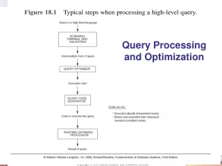
Join Employee Project Join Employee and Project using hash join, … ... Steps in Query Processing SQL query Query Parsing Parse Tree Query Optimization Execution Plan Code Generation Runtime DB Processor Result Code Department of Computer Science and Engineering, HKUST Slide 3
Select Operation • File scan scan all records of the file to find records that satisfy selection condition • Binary search when the file is sorted on attributes specified in the selection condition • Index scan using index to locate the qualified records • Primary index, single record retrieval equality comparison on a primary key attribute with a primary index • Primary index, multiple records retrieval comparison condition <, >, etc. on a key field with primary index • Clustering index to retrieve multiple records • Secondary index to retrieve single or multiple records When would file scan be better than index scan? Department of Computer Science and Engineering, HKUST Slide 4
Composite index EmpNo Age Complete Employee Records 012 25 123 30 Conjunctive Conditions • OP1 AND OP2 (e.g., EmpNo=123 AND Age=30) • Conjunctive selection: Evaluate the condition that has an index created (I.e., that can be evaluated very fast), get the qualified tuples and then check if these tuples satisfy the remaining conditions. • Conjunctive selection using composite index: if there is a composite index created on attributes involved in one or more conditions, then use the composite index to find the qualified tuples • Conjunctive selection by intersection of record pointers: if secondary indexes are available, evaluate each condition and intersect the sets of record pointers obtained. Department of Computer Science and Engineering, HKUST Slide 5
Conjunctive Conditions (cont.) • When there are more than one attribute with an index: • use the one that costs least, and • the one that returns the smallest number of qualified tuple • selectivity of a condition is the number of tuples that satisfy the condition divided by total number of tuples. • The smaller the selectivity, the fewer the number of tuples retrieved, and the higher the desirability of using that condition to retrieve the records. • Disjunctive select conditions: OP1 or OP2 are much more costly: • potentially a large number of tuples will qualify • costly if any one of the condition doesn’t have an index created Department of Computer Science and Engineering, HKUST Slide 6
Join Operation • Join is one of the most time-consuming operations in query processing. • Two-way join is a join of two relations, and there are many algorithms to evaluate the join. • Multi-way join is a join of more than two relations; different orders of evaluating a multi-way join have different speeds • We shall study methods for implementing two-way joins of form R A=B S Department of Computer Science and Engineering, HKUST Slide 7
m tuples in R R S 0005 n tuples in S 0005 0002 0002 0004 0002 0002 0003 0002 m*n checkings 0002 0001 0005 0005 Join Algorithm: Nested (inner-outer) Loop R A=B S • Nested (inner-outer) Loop: For each record r in R (outer loop), retrieve every record s from S (inner loop) and check if r[A] = s[B]. for each tuple r in R do for each tuple s in S do if r.[A] = s[B] then output result end end R and S can be reversed Department of Computer Science and Engineering, HKUST Slide 8
R 0005 index on S S 0005 0002 0002 0004 0002 0002 0003 0002 0002 0001 0005 0005 When One Join Attributes is Indexed • If an index (or hash key) exists, say, on attribute B of S, should we put R in the outer loop or S? Why? • Records in the outer relation are accessed sequentially, an index on the outer relation doesn’t help; • Records in the inner relations are accessed randomly, so an index can retrieve all records in the inner relation that satisfy the join condition. for each tuple r in R do lookup r.[A] in S if found then output result end Department of Computer Science and Engineering, HKUST Slide 9
0001 0002 0002 0002 0002 0002 0002 0004 0003 0005 0005 0005 0005 Sort-Merge Join R A=B S • Sort-merge join: if the records of R and S are sorted on the join attributes A and B, respectively, then the relations are scanned in say ascending order, matching the records that have same values for A and B. • R and S are only scanned once. • Even if the relations are not sorted, it is better to sort them first and do sort-merge join then doing double-loop join. • if R and S are sorted, n + m • if not sorted:n log(n) + m log(m) + m + n Department of Computer Science and Engineering, HKUST Slide 10
0001 0003 0005 0001 0002 0002 0002 0005 0002 0002 0002 0002 0002 0002 0002 0002 0002 0003 0004 0004 0005 0005 0005 0005 0005 0005 Hash Join Method • Hash-join: R and S are both hashed to the same hash file based on the join attributes. Tuples in the same bucket are then “joined”. Department of Computer Science and Engineering, HKUST Slide 11
Hints on Evaluating Joins • Disk accesses are based on blocks, not individual tuples • Main memory buffer can significantly reduce the number of disk accesses • Use the smaller relation in outer loop in nested loop method • Consider if 1 buffer is available, 2 buffers, m buffers • When index is available, either the smaller relation or the one with large number of matching tuples should be used in the outer loop. • If join attributes are not indexed, it may be faster to create the indexes on-the-fly (hash-join is close to generating a hash index on-the-fly) • Sort-Merge is the most efficient; the relations are often sorted already • Hash join is efficient if the hash file can be kept in the main memory Department of Computer Science and Engineering, HKUST Slide 12
Query Optimization • Give a relational algebra expression, how do we transform it to a more efficient one? • Use the query tree as a tool to rearrange the operations of the relational algebra expression Department of Computer Science and Engineering, HKUST Slide 13
A Query Tree ProjNo,DeptNo,EmpName,Address,Birthdate (3) MgrNo=EmpNo Employee (2) DeptNo=DeptNo Department ProjLocation=‘Stafford’ (1) Empolyee (EmpNo, EmpName, Address, Birthdate, DeptNo) Department (DeptNo, DeptName, MgrNo) Project (ProjNo, ProjName, ProjLocation, DeptNo) WorksOn (EmpNo, ProjNo, Hours) Project Department of Computer Science and Engineering, HKUST Slide 14
Structure and Execution of a Query Tree • A query tree is a tree structure that corresponds to a relational algebra expression by representing the input relations as leaf nodes and the relational algebra operations as internal nodes of the tree • An execution of the query tree consists of executing an internal node operation whenever its operands are available and then replacing that internal node by the relation that results from executing the operation Department of Computer Science and Engineering, HKUST Slide 15
Heuristics for Optimizing a Query • A query may have several equivalent query trees • A query parser generates a standard canonical query tree from a SQL query tree • Cartesian products are first applied (FROM) • then the conditions (WHERE) • and finally projection (SELECT) Department of Computer Science and Engineering, HKUST Slide 16
ProjNo,DeptNo,EmpName,Address,Birthdate ProjLocation=‘Stafford’ AND MgrNo=EmpNo AND DeptNo=DeptNo, Employee Project Department Heuristics for Optimizing a Query select ProjNo, DeptNo, EmpName, Address, Birthdate fromProject, Department, Employee where ProjLocation=‘Stafford’ and MrgNo=EmpNo and Department.DeptNo=Employee.DeptNo The query optimizer transforms this canonical query into an efficient final query Department of Computer Science and Engineering, HKUST Slide 17
EmpName ProjName=‘Aquarius’ AND Project.ProjNo=Project.ProjNo AND Employee.EmpNo=WorksOn.EmpNo AND Birthdate > ‘DEC-31-1957’ Project Employee WorksOn Example Find the names of employees born after 1957 who work on a project named ‘Aquarius’ select EmpName from Employee, WorksOn, Project where ProjName=‘Aquarius’ AND Project.ProjNo=WorksOn.ProjNo AND Employee.EmpNo = WorksOn.EmpNo AND Birthdate >‘DEC-31-1957’ WorksOn (EmpNo, ProjNo, Hours) Department of Computer Science and Engineering, HKUST Slide 18
EmpName ProjNo=ProjNo EmpNo=EmpNo ProjName=‘Aquarius’ Project Birthdate > ‘dec-31-1957’ WorksOn Employee Expensive due to large size of Employee Example Push all the conditions as far down the tree as possible Department of Computer Science and Engineering, HKUST Slide 19
EmpName EmpNo=EmpNo ProjNo=ProjNo Birthdate > ‘dec-31-1957’ Employee PNAME=‘Aquarius’ WorksOn Project Example Rearrange join sequence according to estimates of relation sizes Department of Computer Science and Engineering, HKUST Slide 20
Only need EmpNo attribute from Employee and WorksOn and EmpName from Employee EmpName EmpNo= EmpNo Only need ProjNo attribute from Project and WorksOn ProjNo= ProjNo Birthdate > ‘dec-31-1957’ ProjName=‘Aquarius’ WorksOn Employee Project Example Replace cross products and selection sequence with a join operation Department of Computer Science and Engineering, HKUST Slide 21
Example LNAME Push projection as far down the query tree as possible EmpNo = EmpNo EmpNo EmpNo, EmpName ProjNo= ProjNo Birthdate > ‘dec-31-1957’ ProjNo EmpNo, ProjNo Employee ProjName=‘Aquarius’ WorksOn Project Department of Computer Science and Engineering, HKUST Slide 22
Transformation Rules • 1. Cascade of : A conjunctive selection condition can be broken up into a cascade (sequence) of individual operations: • c1 AND c2 AND...AND cn(R) c1(c2(...(cn(R))..)) • 2. Commutativity of :c1(c2(R)) c2(c1(R)) • 3. Cascade of : • List1(List2(... (Listn(R))... )) List1(R)if List1 is included in List2…Listn; result is null if List1 is not in any of List2…Listn Department of Computer Science and Engineering, HKUST Slide 23
Transformation Rules (Cont.) • 4. Commuting with : if the projection list List1 involves only attributes that are in condition c • List1(c(R)) c(List1(R)) • 5. Commutivity of JOIN or : R S S R • 6. Commuting with JOIN: if all the attributes in the selection condition c involve only the attributes of one of the relations being joined, say, R • c(R S) (c(R)) S Department of Computer Science and Engineering, HKUST Slide 24
Transformation Rules (Cont.) • 7. Commuting with JOIN: if List can be separated into List1 and List2 involving only attributes from R and S, respectively, and the join condition c involves only attributes in List: • List(R c S) (List1(R) cList2(S)) • 8. Commuting set operations: and are commutative • 9. JOIN, , , are associative • 10. distributes over , , • c (R S) c(R) c(S) • 11. distributes over • List (R S) (List(R) List(S)) Department of Computer Science and Engineering, HKUST Slide 25
Heuristic Algebraic Optimization • Use rule 1 to break up any operation with conjunctive conditions into a sequence of operations • Use rules 2, 4, 6, and 10 concerning commutativity of with other operations to move each operation as far down the query tree as possible based on the attributes in the operations • Use rule 9 concerning associativity of binary operations to rearrange the leaf nodes of the tree so that the leaf node relations with the most restrictive operations are executed Department of Computer Science and Engineering, HKUST Slide 26
Heuristic Algebraic Optimization (Cont.) • Combine sequences of Cartesian product and operation representing a join condition into single JOIN operations • Use rules 3, 4, 7, and 11 concerning the cascading of and commuting with other operations, break down a and move the projection attributes down the tree as far as possible • Identify subtrees that represent groups of operations that can be executed by a single algorithm (select/join followed by project) Department of Computer Science and Engineering, HKUST Slide 27
Estimation of the Size of Joins • The Cartesian product r s contains nrns tuples; each tupleoccupies sr + ss bytes. • If R S = , then r s is the same as r x s. • If R S is a key for R, then a tuple of s will join with at most one tuple from r; therefore, the number of tuples in r s is no greater than the number of tuples in s.If R S in S is a foreign key in S referencing R, then the number of tuples in r s is exactly the same as the number of tuples in s.The case for R S being a foreign key referencing S is symmetric. R S Matching tuples Department of Computer Science and Engineering, HKUST Slide 28
Example of Size Estimation • In the example query depositor customer, customer-name in depositor is a foreign key of customer; hence, the result has exactly depositor tuples, which is 5000. • Data: R = Customer, S = Depositor customer = 10,000 fcustomer = 25 bcustomer = 10000/25 = 400 depositor = 5,000 fdepositor = 50 bdepositor = 5000/50 = 100 Department of Computer Science and Engineering, HKUST Slide 29
Estimation of the size of Joins • If R S = {A} is not a key for R or S.If we assume that every tuple t in R produces tuples in R S, number of tuples in R S is estimated to be: r s V(A, s) • If the reverse is true, the estimates obtained will be: r sV(A, r) • The lower of these two estimates is probably the more accurate one. Number of distinct values of A in s sV(A, s) R S Department of Computer Science and Engineering, HKUST Slide 30
There are 5,000 tuples in depositor relation but has only 2,500 distinct depositors, so every depositor has two accounts Customer-name is unique Estimation of the size of Joins • Compute the size estimates for depositor customer without using information about foreign keys: • customer = 10,000depositor = 5,000V(customer-name, depositor ) = 2500 V(customer-name, customer ) = 10000 • The two estimates are 5000 * 10000/2500 = 20,000 and 5000 * 10000/10000 = 5000 • We choose the lower estimate, which, in this case, is the same as our earlier computation using foreign keys. Department of Computer Science and Engineering, HKUST Slide 31
Nested-Loop Join (Tuple-Based) • Compute the theta join, r s for each tuple tr in r do begin for each tuple ts in s do begin test pair (tr, ts) to see if they satisfy the join condition if they do, add tr · ts to the result. End end • r is called the outer relation and s the inner relation of the join. • Requires no indices and can be used with any kind of join condition. • Expensive since it examines every pair of tuples in the two relations. • For each tuple in the outer relation (r), loop through all nstuples in the inner relation (s) • Cost is nr x ns Department of Computer Science and Engineering, HKUST Slide 32
no. of bocks in s no. of bocks in r Cost of Nested-Loop Join • If there is enough memory to hold only one block of each relation, the estimated cost is nr * bs + br disk accesses • If the smaller relation fits entirely in memory, use it as the inner relation. This reduces the cost estimate to br + bs disk accesses. • br + bs is the minimum possible cost to read R and S once • Putting both relations in memory won’t reduce the cost further For each tuple in r, S has to be read into buffer, bs disk accesses br disk accesses to load R into buffer R S Department of Computer Science and Engineering, HKUST Slide 33
Nested-Loop Join with Buffers (Still Tuple Based) • The algorithm is the same as in the previous slide • Tuples are fetched and compared one by one according to the double loop • OS or DBMS fetches a tuple from buffer if it is already there For each tuple in r, S has to be read into buffer, bs disk accesses br disk accesses to load R into buffer R S • At this point, one block of r is read, and the first r-tuple has been compared to 3 s-tuples (1 block of s) Department of Computer Science and Engineering, HKUST Slide 34
Nested-Loop Join with Buffers (Still Tuple Based) br disk accesses to load R into buffer R S • At this point, the first r-tuple has been compared to 6 s-tuples • The next step begins with the 2nd tuple in r’s buffer; no access to r on disk is needed; however, the s-tuples have to be read from disk again • Total cost = nr * bs + br disk accesses Department of Computer Science and Engineering, HKUST Slide 35
Rewriting the Nested-Loop Join • To make use of the buffer efficiently, the algorithm has to be buffer-aware • for each block Br in r do beginfor each block Bs in s do begin Do all tuples in Br and Bs: Br Bs end end R S • Total cost = br * bs + br disk accesses Department of Computer Science and Engineering, HKUST Slide 36
Rewriting the Nested-Loop Join • To make use of the buffer efficiently, the algorithm has to be rewritten • for each block Br in r do begin for each block Bs in s do begin Do all tuples in Br and Bs: Br Bs end end • Total cost = br * bs + br disk accesses R S Department of Computer Science and Engineering, HKUST Slide 37
Rewriting the Nested-Loop Join • To make use of the buffer efficiently, the algorithm has to be rewritten • for each block Br in r do begin for each block Bs in s do begin Do all tuples in Br and Bs: Br Bs end end • Total cost = br * bs + br disk accesses R S Department of Computer Science and Engineering, HKUST Slide 38