Download
1 / 13
130 likes | 265 Vues
Can we use total field magnetics to find buried pit houses beneath layers of volcanic ash?. Visible pit houses at Bridge River, B.C. (Prentiss et al., 2009). Approach, constraints and thoughts:

E N D
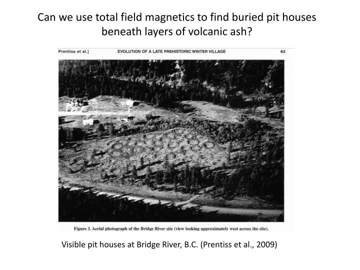
Can we use total field magnetics to find buried pit houses beneath layers of volcanic ash? Visible pit houses at Bridge River, B.C. (Prentiss et al., 2009)
Approach, constraints and thoughts: • The site, Anangula in the Aleutian Islands, has up to two meters of volcanic ash burying some of the pit houses Can we use total field magnetics to find buried pit houses beneath layers of volcanic ash?
Bridge River Study: vertical magnetic gradient The vertical magnetic gradient observations from Prentiss et al. (2009) provide an analog to model similar features in the Aleutians. The result helps confirm the likely success of magnetic exploration to map the layout of the site. Note that the observed values of vertical magnetic gradient are very high with a range of about 200 nt/m. A portion of the amplitude of the circular highs (red rings) is probably due to the excavated soil.
Vertical gradient magnetometer observations from the Bridge River, British Columbia site provide an analog for modeling
To test a worst case situation produce a signal much less than that of the Bridge River results Use forward magnetic models of truncated vertical cylinders
Signal range is about 25% of that for the Bridge River vertical gradient observations Use forward magnetic models of truncated vertical cylinders
Total Field Intensity (TMI) and Vertical Gradient of the Total Field:these anomalies are calculated over simulated pit houses Pit houses modeled as vertical cylinders 2m tall, with radius = 6m, and tops at the surface. Amplitudes of anomalies are scaled so that the range of the vertical gradient is about 25% of the anomalies from Bridge River. This tests a weaker case. Some measure the vertical gradient in the field but it can be calculated from total field observations as one type of edge detector (aka image enhancement).
RecalculatedTMI and Vertical Gradient Anomalies: simulated pit houses are now 2 meters below the surface The range of the vertical gradient is now reduced to about 10 nt, or 5% of the values measured at Bridge River. This is due to lowering the top of the modeled pit houses to 2m below the surface. The anomalies are still very strong.
Contaminate the weak forward signal with substantial noise:determine if we can still recover signal Simulated Fractal Noise: Amplitude ~Equal to the TMI Signalsignal/noise ~ 1 !
Random (1/f2) magnetization (A/m) simulating very variable soil properties Magnetic field (TMI) calculated from the 1/f2 distribution of magnetization Adding this magnetic field to that for the two meter deep pit houses will simulate a ‘bad’ field situation. The noise (+/-20 nt) is a bit greater than the TMI’s range (+/-15nt).
Add the Fractal Noise to the Signal From 2m Deep Pit Houses: a field situation with an extremely low signal to noise ratio The general location of the deep pit houses, even though greatly obscured by the noise, is still apparent in the total field anomaly even without any processing. The location of the pit houses is very difficult to distinguish in the vertical gradient anomaly. This is because the vertical gradient is a high pass frequency operator and biases against the signal from the deep pit houses.
Post-processing Enhances the TMI Anomalies Deep equivalent magnetic layer after separating shallow source components with matched filtering Maxima of the horizontal gradient of the pseudogravity transform of the TMI; highs estimate edges of sources. Even in this low signal/noise situation the pit houses standout.
Summary Pit house model parameters for a pretty bad (if not worse) case field scenario: • House diameter = 6 meters; depth to top = 2 meters • Surface magnetic anomalies scaled to 25% of Bridge River vertical gradients • After burial to two meters signal amplitude is about 5% of Bridge River values • Two meter layer of fractal noise added to signal to simulate volcanic soils • Model signal to noise ratio ~ 1 • 1 meter spacing of observations; they would be at 0.1 meter along lines in the field. The modeled situation is quite pessimistic relative to known results at Bridge River. Regardless, the pit houses are still very apparent. If the Bridge River results are at all characteristic, the situation at Anangula in the Aleutian Islands could easily be much better than this model.