Generalization and Specialization of Kernelization
Generalization and Specialization of Kernelization. Daniel Lokshtanov. We. Kernels. ¬. ∃. Kernels. Why?. What’s Wrong with Kernels (from a practitioners point of view). Only handles NP-hard problems. Don’t combine well with heuristics . Only capture size reduction .

Generalization and Specialization of Kernelization
E N D
Presentation Transcript
Generalization and Specialization of Kernelization Daniel Lokshtanov
We Kernels ¬ ∃ Kernels Why?
What’s Wrong with Kernels(from a practitioners point of view) • Only handles NP-hard problems. • Don’t combine well with heuristics. • Only capture size reduction. • Don’t analyze lossy compression. Doing something about (1) is a different field altogether. Some preliminary work on (4) high fidelity redections This talk; attacking (2)
”Kernels don’t combine with heuristics” ?? Kernel mantra; ”Never hurts to kernelize first, don’t lose anything” We don’t lose anything if after kernelization we will solve the compressed instance exactly. Do not necessarily preserveapproximate solutions.
Kernel In this talk, parameter = solution size / quality I,k I’,k’ Solution of size ≤ k Solution of size ≤ k’ ?? Solution of size 1.2k Solution of size 1.2k’
Known/Unknown k Don’t know OPT in advance. Solutions: • The parameter k is given and we only care whether OPT ≤ k or not. • Try all values for k. • Compute k ≈ OPT by approximation algorithm. Overhead If k > OPT, does kernelizing with k preserve OPT?
Buss kernel for Vertex Cover Vertex Cover: Find S ⊆ V(G) of size ≤ k such that every edge has an endpoint in S. • Remove isolated vertices • Pick neighbours of degree 1 vertices into solution (and remove them) • Pick degree > k vertices into solution and remove them. Reduction rules are independent of k. Proof of correctness transforms any solution, not only any optimal solution.
Degree > k rule Any solution of size ≤ k must contain all vertices of degree > k. We preserve all solutions of size ≤ k. Lose information about solutions of size ≥ k.
Buss’ kernel for Vertex Cover • Find a 2-approximate solution S. • Run Buss kernelization with k = |S|. I,k’ I,k Solution of size 1.2k’ + (k-k’) ≤ 1.2k Solution of size 1.2k’
Buss’ - kernel - Same size as Buss kernel, O(k2), up to constants. - Preserves approximate solutions, with no loss compared to the optimum in the compression and decompression steps.
NT-Kernel In fact the Nemhauser Trotter 2k-size kernel for vertex cover already has this property – the crown reduction rule is k-independent! Proof: Exercise
Other problems For many problems applying the rules with a value of k preserves all ”nice” solutions of size ≤ k approximation preserving kernels. Example 2: Feedback Vertex Set, we adapt a O(k2) kernel of [T09].
Feedback Vertex Set FVS: Is there a subset S ⊆ V(G) of size ≤ k such that G \ S is acyclic? R1: Delete vertices of degree 0 and 1. R2: Replace degree 2 vertices by edges. R3: If v appears in > k cycles that intersect only in v, select v into S. R1 & R2 preserve all reasonable solutions R3 preserves all solutions of size ≤ k
Feedback Vertex Set R4 (handwave): If R1-R3 can’t be applied and there is a vertex x of degree > 8k, we can identify a set X such that in any feedback vertex set S of size ≤ k, either x ∈ S or X ⊆ S. R4 preserves all solutions of size ≤ k
Feedback Vertex Set Kernel Apply a 2-approximation algorithm for Feedback Vertex Set to find a set S. Apply the kernel with k=|S|. Kernel size is O(OPT2). Preserves approximate solutions, with no loss compared to the optimum in the compression step.
Remarks; If we don’t know OPT, need an approximation algorithm. Most problems that have polynomial kernels also have constant factor or at least Poly(OPT)approximations. Using f(opt)-approximations to set k results in larger kernel sizes for the approximationpreserving kernels.
Right definition? Approximation preserving kernels for optimization problems, definition 1: I I’ |I’I≤ poly(OPT) OPT’ OPT Poly time Poly time c*OPT c*OPT’
Right definition? Approximation preserving kernels for optimization problems, definition 2: I I’ |I’I≤ poly(OPT) OPT’ OPT Poly time Poly time OPT + t OPT’ + t
What is the right definition? Definition 1 captures more, but Definition 2 seems to capture most (all?) positive answers. Exist other reasonable variants that are not necessarily equivalent.
What do approximation preserving kernels give you? When do approximation preserving kernels help in terms of provable running times? If Π has a PTAS or EPTAS, and an approximation preserving kernel, we get (E)PTASes with running time f(ε)poly(OPT) + poly(n) or OPTf(ε) + poly(n).
Problems on planar (minor-free) graphs Many problems on planar graphs and H-minor-free graphs admit EPTAS’s and have linear kernels. Make the kernels approximation preserving? These Kernels have onlyone reduction rule; the protrusion rule. (to rule them all)
Protrusions A set S ⊆ V(G) is an r-protrusion if • At most r vertices in S have neighbours outside S. • The treewidth of G[S] is at most r.
Protrusion Rule A protrusion rule takes a graph G with an r-protrusion S of size > c, and outputs an equivalent instance G’, with V(G’) < V(G). Usually, the entire part G[S] is replaced by a different and smaller protrusion that ”emulates” the behaviour of S. The constant c depends on the problem and on r.
Kernels on Planar Graphs [BFLPST09]: For many problems, a protrusion rule is sufficient to give a linear kernel on planar graphs. To make these kernels apx-preserving, we need an apx-preserving protrusion rule.
Apx-Preserving Protrusion Rule S I I’ |I’I< I OPT OPT’≤ OPT Poly time Poly time OPT + t OPT’ + t
Kernels on Planar Graphs [BFLPST09]: • If a problem has finite integer index it has a protrusion rule. • Simple to check sufficient condition for a problem to have finite integer index. Finite integer index is not enough for apx-preserving protrusion rule. But the sufficient condition is!
t-boundaried graphs A t-boundaried graph is a graph G with t distinguished vertices labelled from 1 to t. These vertices are called the boundary of G. G can be colored, i.e supplied with some vertex/edge sets C1,C2… C1 C2
Gluing Gluing two colored t-boundaried graphs: (G1,C1,C2) ⊕ (G2,D1,D2) (G3, C1∪ D1, C2∪ D2)means identifying the boundary vertices with the same label, vertices keep their colors. 1 D2 1 1 C1 C1 D2 2 D1 C2 C2 D1 2 2 3 3 3
Canonical Equivalence For a property Φ of 1-colored graphs we define the equivalence relation ≣Φ on the set of t-boundaried c-colored graphs. (G1,X1) ≣Φ(G2,X2) ⇔ For every (G’, X’): Φ(G1⊕G’, X1∪X’) ⇔ Φ(G2⊕G’, X2∪ X’) Can also define for 10-colorable problems in the same way
Canonical Equivalence (G1,X) ≣Φ(G2,Y) means ”gluing (G1,X) onto something has the same effect as gluing (G2,Y) onto it” Y2 1 Z2 1 1 X1 Y1 2 Z1 X2 2 2 3 3 3
Finite State Φ is finite state if for every integer t, ≣Φ has a finite number of equivalence classes on t-boundaried graphs. Note: The number of equivalence classes is a function f(Φ,t) of Φ and t.
Variant of Courcelle’s Theorem Finite State Theorem (FST): If Φ is CMSOL-definable, then Φ is finite state. Quantifiers:∃ and ∀ for variables for vertex sets and edge sets, vertices and edges. Operators: = and ∊ Operators: inc(v,e) and adj(u,v) Logical operators: ∧, ∨ and ¬ Size modulo fixed integers operator: eqmodp,q(S) EXAMPLE: p(G,S) = “S is an independent set of G”:p(G,S) = ∀u, v ∊ S, ¬adj(u,v)
CMSOL Optimization Problemsfor colored graphs Φ-Optimization Input: G, C1, ... Cx Max / Min |S| So that Φ(G, C1, Cx, S) holds. CMSOL definable proposition
Sufficient Condition [BFLPST09]: • If a CMSO-optimization problem Π is strongly monotone Π has finite integer index it has a protrusion rule. Here: • If a CMSO-optimization problem Π is strongly monotone Πhas apx-preservingprotrusion rule.
Signatures (for minimization problems) |SG1| = 2 H1 2 Choose smallest S ⊆ V(G) to make Φ hold SH1 |SG2|=5 G H2 |SG3|=1 5 SH2 H3 Intuition: f(H,S) returns the best way to complete in G a fixed partial solution in H. 1 SH3
Signatures (for minimization problems) The signature of a t-boundaried graph G is a function fG with Input:t-boundaried graph H and SH ⊆ V(H) Output:Size of the smallest SG ⊆ V(G) such that Φ(G ⊕ H, SG ∪ SH) holds. Output:∞ if SG does not exist.
Strong Monotonicity(for minimization problems) A problem Π is strongly monotone if for any t-boundaried G, there is a vertex set Z ⊆ V(G) such that |Z| ≤ fG(H,S) + g(t) for an arbitrary function g. Signature of G, evaluated at (H,S) Size of the smallest S’ ⊆ V(G) such that S’ ∪ S is a feasible solution of G ⊕ H
Strong monotonicity - intuition Intuition:A problem is strongly monotone if for any t-boundaried G there ∃ partial solution S that can be glued onto ”anything”, and S is only g(t) largerthan the smallest partial solution in G.
SuperStrongMonotonicityTheorem Theorem: If a CMSO-optimization problem Π is strongly monotone, then it has apx-preserving protrusion rule. Corollary: All bidimensional’, strongly monotoneCMSO-optimization problems Πhave linear size apx-preserving kernels on planar graphs.
Proof of SSMT Lemma 1: Let G1 and G2 be t-boundaried graphs of constant treewidth, f1 and f2 be the signatures of G1 and G2, and c be an integer such that for any H, SH ⊆ V(H):f1(H,SH) + c = f2(H,SH). Then: Decrease size by c Feasible solution Z2 Feasible solution Z1 Poly time Increase size by c G2 ⊕ H G1 ⊕ H Poly time
Proof of Lemma 1 G1 H Decrease size by c Poly time? G2 Constant treewidth! H
Proof of SSMT Lemma 2: If a CMSO-min problem Π is strongly monotone, then: For every t there exists a finite collection F of t-boundaried graphs such that: For every G1, there is a G2 ∈ F and c ≥ 0 such that: For any H, SH ⊆ V(H):f1(H,SH) + c = f2(H,SH).
SSMT = Lemma 1 + 2 Keep a list F of graphs t-boundaried graphs as guaranteed by Lemma 2. Replace large protrusions by the corresponding guy in F. Lemma 1 gives correctness.
Proof of Lemma 2 Signature value G2 G1 ≤ g(t) (H1, S1) (H2, S2) (H3, S3) (H4, S4) (H5, S5) (H6, S6) (H7, S7) (H8, S8) ...
Proof of Lemma 2 Only a constant number of finite, integer curves that satisfy max-min ≤ t (up to translation). Infinite number of infinite such curves. Since Π is a min-CMSO problem, we only need to consider the signature of G on a finite number of pairs (Hi,Si).
SuperStrongMonotonicityTheorem Theorem: If a CMSO-optimization problem Π is strongly monotone, then it has apx-preserving protrusion rule. Corollary: All bidimensional’, strongly monotoneCMSO-optimization problems Πhave linear size apx-preserving kernels on planar graphs.
Recap Approximation preserving kernels are much closer to the kernelization ”no loss” mantra. It looks like most kernels can be made approximation preserving at a small cost. Is it possible to prove that some problems have smaller kernels than apx-preserving kernels?
What I was planning to talk about, but didn’t. ”Kernels” that do not reduce size, but rather reduce a parameter to a function of another in polynomial time. • This IS pre-processing • Many many examples exist already • Fits well into Mike’s ”multivariate” universe.