Download
1 / 71
710 likes | 903 Vues
The scientific case for a photon-photon collider. Edoardo Milotti Università e INFN-Sezione di Trieste milotti@ts.infn.it LNF – 14/12/2012. The scientific case for a (low-energy) photon-photon collider. Edoardo Milotti Università e INFN-Sezione di Trieste milotti@ts.infn.it

E N D
The scientific case for a photon-photon collider Edoardo Milotti Università e INFN-Sezione di Trieste milotti@ts.infn.it LNF – 14/12/2012
The scientific case for a (low-energy) photon-photon collider Edoardo Milotti Università e INFN-Sezione di Trieste milotti@ts.infn.it LNF – 14/12/2012
Given the present value of the Higgs mass, a 70+70 GeV photon-photon collider would suffice for a very rich physics program. However, for all its potential, a high-energy photon-photon collider has not yet been built. A low-energy photon-photon collider could lead to the necessary technology developments and prepare the ground for a higher energy complex, while still providing a rich testing ground for QED, and, more generally, QFT.
QED is a successful theory but there still are unsolved pitfalls. Possibly, the most notable one is the “cosmological constant problem”.
The QFT vacuum: modes and energy density of the EM vacuum Number of modes of em radiation in a box of volume V
energy density = (energy per mode)·(number of modes)/(volume of box) EM energy density (integrate over all frequencies) number of polarization states density of modes energy of one mode (ground-level of quantum oscillator)
This result diverges at high frequency ultraviolet cutoff GZK cutoff at about 1010 GeV (highest-energy known photons) Pierre Auger collaboration, Phys. Lett. B 685 (2010) 239 A HUGE NUMBER !!! about 1041 times the measured nuclear density
We can be even more ambitious and take the Planck energy for the ultraviolet cutoff A HUMONGOUS NUMBER !!!
Contributions to vacuum energy density (zero point energy) from other fields • Bosons (spin 1 particles): • photon: 2 polarizations • gluons: 8 types of gluons, 2 polarizations • Ws and Z bosons: 3 bosons, 3 polarizations (massive force carriers) • total: 27 boson degrees of freedom • Fermions (spin 2 particles): • 6 massive quark fields, 2 polarizations • 3 massive lepton fields, 2 polarizations • 3 neutrino fields • total: 21 fermion degrees of freedom • Contribution of each degree of freedom total = AN EVEN LARGER NUMBER !!! fermionic d.o.f.’s give a negative contribution
Supersymmetry (doubling of all bosonic and fermionic degrees of freedom) would thus solve the problem, leading to a vanishing energy density, but only when supersymmetry is not broken. Therefore the problem of a high energy density of vacuum would still persist at low energy, even in a supersymmetric world.
Using the density of flat universe (critical density) as upper bound for the vacuum energy density we find while using the radiation density alone we find This stronger bound is 113 orders of magnitude smaller than the previously estimated value. Other estimates put this ratio at 120 orders of magnitude. This is the “cosmological constant problem”. The QFT vacuum is a BIG problem !!!
This problem has actually been with us for a long time now. It was already there after Dirac wrote his equation, and invented the Dirac sea, where an infinite number of degrees of freedom are occupied by unseen particles.
soon after Dirac’s theory of the positron, it was understood that this could lead to photon-photon scattering ... Euler-Heisenberg and Weisskopf (EHW) Lagrangian
E positive energy states +mec2 -mec2 filled negative energy states
E positive energy states e- +mec2 creation-destruction of electron-positron pair -mec2 e+ filled negative energy states the time-energy uncertainty principle allows the creation of electron-positron pairs for very short times
E positive energy states electron +mec2 creation of electron-positron pair -mec2 positron (hole) filled negative energy states E creation of virtual electron-positron pair photon scatters off virtual electron virtual electron radiates and returns to negative energy state electron and positron annihilate +mec2 2 3 -mec2 1 4
E positive energy states electron +mec2 creation of electron-positron pair Not yet observed! strong external electric field E -mec2 positron (hole) filled negative energy states Extraction of electron pairs from vacuum under the action of a strong electric field: this is a sort of tunnelling (Schwinger effect). Estimate of critical field: charge separation energy ≈ electron rest energy
This Lagrangian contains the two invariants • where • The generic Lagrangian which is • Lorentz invariant • parity invariant • gauge invariant • has no derivatives of the fields of order greater than 1 (locality constraint) • has the form
the QED result (Schwinger Lagrangian) is Other Lagrangians are possible and lead to different c’s, e.g., the Born-Infeld Lagrangian this b is a max B field intensity in BI theory as in the EHW Lagrangian in the EHW Lagrangian there is a 7 here
The full (classical) BI Lagrangian is and it incorporates a “maximum field” b, thereby automatically resolving the problem of divergent quantities (no regularization-renormalization of charge is necessary)
it is interesting to notice that from the BI Lagrangian we find and therefore when fields are present, vacuum becomes anisotropic (Denisov, PRD 61 (2000) 036004)
A few consequences of the phenomenological EHW Lagrangian • electric and magnetic birefringence of vacuum • low-energy photon-photon scattering • approximate description of Delbrück scattering • approximate description of photon-splitting
Photon-photon scattering (first complete calculation by Karplus and Neuman in 1950-51, further refinements by De Tollis and collaborators in the following years) electromagnetic polarization tensor the em pol. tensor is completely symmetric with respect to indices and momenta and is divergenceless and P-invariant tensor must be regularized
Differential cross-section Polarization dependent amplitude
each polarization-dependent amplitude is associated to six different diagrams the calculation involves several complex integrals, however it has been simplified considerably by De Tollis who introduced double-dispersion techniques in 1964
finally, for , the differential photon-photon scattering cross-section is This cross-section is derived from a genuine non-linear QED effect (loop) and its value is critically dependent on the regularization procedure. The importance of regularization has recently been emphasized by the a couple of wrong preprints, that claimed that the photon-photon cross section is actually (see N. Kanda, arXiv:1106.0592, and T. Fujita and N. Kanda, arXiv:1106.0465, and the refutation by Y. Liang and A. Czarnecki, arXiv:1111.6126)
Why this discrepancy? • The origin of the error lies in neglecting the regularization-renormalization of the scattering amplitudes • Kanda and Fujita argued that there is no need of regularization-renormalization because the unrenormalized amplitudes are finite • However the regularization-renormalization process breaks the symmetry of the QED Lagrangian, and cannot be neglected even in this finite case • Although the issue is not quite clear, it can be conjectured that this is associated to the ABJ chiral anomaly
The origin of the chiral anomaly seems to lie very deep in the structure of spacetime and of quantum vacuum. The standard approach (R. W. Jackiw, Int. J. Mod. Phys. A, 25(2010) 659)Both the massless and the massive Dirac equations share a common symmetry: global gauge transformation
when we introduce the matrix we find that the new matrix anticommutes with the other gamma-matrices. We can also construct chiral projection matrices: which select chiral components of the field: This leads to decoupled equations for the massless case
Chiral charges and currents can also be defined: and in the massless case, the charges are separately conserved. The axial vector current also satisfies a continuity equation, and the axial charge is conserved. This is related to the new gauge transformation
The same is not true for the massive case, where a mixing remains On the other hand, if we include an external vector field in the massless equation the previous gauge symmetries continue to hold, and can even be generalized to local gauge symmetries, if the vector field is also transformed
However, even the massless case has problems with the gauge symmetries when we step from classical functions to quantum fields. • With quantum fields the fundamental quantization condition for Fermi-Dirac fields must hold • This implies that • there is a singularity at the same space-time point • since charges and currents are defined by bilinears at the same space-time point, they are ill-defined • a regularization/renormalization procedure is required • every regularization/renormalization procedure in the presence of the vector field, breaks symmetries present at the classical level • one or the other gauge symmetry is broken at the quantum level • the usual choice is to abandon axial symmetry
2. Simple physical view (A. Widom and Y. Srivastava, Am. J. Phys. 56 (1988) 824) 1-dimensional, accelerated motion (external field E) positive energy states +mec2 -mec2 negative energy states
overall density of states summed over all momenta Therefore the induced current has the rate of change Since, in this 1D model then the equation for the rate of change of the current becomes linear charge density vector potential
finally this leads to the anomaly equation in 1+1 dimensions A simple extension of this line of reasoning finally leads to the 3+1 dimensional anomaly equation (Schwinger’s equation)
3. Further connections and conjectures • Quantum anomalies are related to the topological properties of space: there is a deep connection with the Atiyah-Singer index theorem (where the index is closely related to the winding number and therefore to the connectivity of space) • A derivation of the chiral anomaly by means of path integrals (Fujikawa, PRL 42 (1979) 1195; PRD 21 (1980) 2848; PRD 22 (1980) 1499; PRL 44 (1980) 1733; PRD 23 (1981) 2262) further indicates a connection with quantum paths • A recent paper by Bender and Hook (“Quantum tunneling as a classical anomaly”, J. Phys. A: Math. Theor. 44 (2011) 372001) further points to an intriguing connection of anomalies with paths and with the nature of space • A tantalizing hint: the Green-Schwartz mechanism cancels anomalies in string theory (Phys. Lett. B149 (1984) 117)
The PVLAS experiment: started back at CERN in the ’80’s An attempt to unravel the mysteries of QFT vacuum, trying a direct measurement of the predicted birefringence
New prototype setup in the Phys. Dept. of the University of Ferrara
The observed birefringence can be related to the low-energy photon-photon cross-section using the optical theorem (for details see, Haïssinski et al. LAL 06-140 (2006), PVLAS Collaboration, PRD 78 (2008) 032006) We start from the relationship between index of refraction and forward scattering amplitude then we note that
Results obtained with the old PVLAS apparatus are published in PRD 78 (2008) 032006) With the new test apparatus we improve on that limit and find while the QED prediction is
PVLAS is an extremely challenging and difficult experiment, however the cross-section for photon-photon scattering grows fast: could we aim at the direct detection of photon-photon scattering? Low-energy cross-section
peak cross-section, ≈1.6 µbarn at cross-section for unpolarized initial state (average over initial polarizations)
approximate differential cross-section for low-energy photons (Eγ < 0.7 me) (averaged over initial polarizations, summed over final) parallel initial polarizations