Download
1 / 30
300 likes | 463 Vues
ADAPTIVE AUGMENTED CONTROL OF UNMANNED ROTORCRAFT VEHICLES C.L. Bottasso , R. Nicastro , L. Riviello , B. Savini Politecnico di Milano AHS International Specialists' Meeting on Unmanned Rotorcraft Chandler, AZ, January 23-25, 2007. Rotorcraft UAVs at PoliMI.

E N D
ADAPTIVE AUGMENTED CONTROL OF UNMANNED ROTORCRAFT VEHICLESC.L. Bottasso, R. Nicastro, L. Riviello, B. SaviniPolitecnico di MilanoAHS International Specialists' Meeting onUnmanned Rotorcraft Chandler, AZ, January 23-25, 2007
Rotorcraft UAVs at PoliMI • Low-cost platform for development and testing of navigation and control strategies (including vision, flight envelope protection, etc.); • Vehicles: off-the-shelf hobby helicopters; • On-board control hardware based on PC-104 standard; • Bottom-up approach: everything is in-house developed (Inertial Navigation System, Guidance and Control algorithms, Linux-based real-time OS, flight simulators, etc. etc.)
Outline • Non-linear model predictive control; • Reference Augmented Predictive Control (RAPC): motivations; • Reference Augmented Model Identification; • Reference Augmented Neural Control; • Results; • Conclusions and outlook.
UAV Control Architecture Hierarchical three-layer control architecture (Gat 1998): • Strategic layer: assign mission objectives (typically relegated to a human operator); • Tactical layer: generate vehicle guidance information, based on input from strategic layer and sensor information; • Reflexive layer: track trajectory generated by tactical layer, control, stabilize and regulate vehicle. • In this paper: Adaptive Non-linear Model Predictive Control. Vision/sensor range Obstacles Target
( ) ¤ ¢ T T ( ) ( ) ( ) ( ) ( ) ¤ ¤ ¤ ¤ Q R L ¡ ¡ + ¡ ¡ y u y y y y u u u u = ; T + t Z 0 p ( ) d J L i t y u m n = ; u x y t ; ; 0 ( ) [ ] f _ T 0 t t t t + 2 x x u s : = 0 0 p . . ; ; ; ( ) t x x = 0 0 ( ) [ ] T t t t + 2 y g x = 0 0 p ; Non-Linear Model Predictive Control • Non-linear Model Predictive Control (NMPC): • Find the control action which minimizes an index of performance, by predicting the future behavior of the plant using a non-linear reduced model. • - Reduced model: • - Initial conditions: • - Output definition: • Cost: • with desired goal outputs and controls. • Stability results: Findeisen et al. 2003, Grimm et al. 2005.
Model-Adaptive Predictive Control Receding horizon control: Prediction window Prediction window Tracking cost Tracking cost Prediction window Tracking cost Goal trajectory Prediction error Prediction error Steering window Steering window Prediction error Plant response Predictive solutions Steering window 1. Tracking problem 2. Steering problem 3. Reduced model update
Motivation • For any given problem: wealth of knowledge and legacy methods which perform reasonably well; • Quest for better performance/improved capabilities: undesirable and wasteful to neglect valuable existing knowledge; • Reference Augmented Predictive Control (RAPC): exploit available legacy methods, embedding them in a non-linear model predictive control framework. • Specifically: • Model: augment flight mechanics rotorcraft models (BEM+inflow theories) to account for unresolved or unmodeled physics; • Control: design a non-linear controller augmenting linear ones (LQR) which are known to provide a minimum level of performance about certain linearized operating conditions.
Outline • Non-linear model predictive control; • Reference Augmented Predictive Control (RAPC): motivations; • Reference Augmented Model Identification; • Reference Augmented Neural Control; • Results; • Conclusions and outlook.
Reference Augmented Model Identification • Goal: • Develop reduced model capable of predicting the behavior of the plant with minimum error (same outputs when subjected to same inputs); • Reduced model must be self-adaptive (capable of learning) to adjust to varying operating conditions. Prediction (tracking) window Prediction error to be minimized Steering window Predictive solutions
e e e e e e d d 6 u x x x x u u u x x u u = = = = ; ; . ; ( ( ) ) ( ) f f d _ _ 0 x x x u x u x u = = f f r e r e ; ; ; ; ; : ; Reference Augmented Model Identification • Neural augmented reference model: • reference (problem dependent) analytical model, • Remark: reference model will not, in general, ensure adequate predictions, i.e. • when = system states/controls, • = model states/controls. • Augmented reference model: • where is the unknown reference model defect that ensures • when • Hence, if we knew , we would have perfect prediction capabilities.
T T T T ( ( ) ( ( ) ) ( ) ) d i Á Á b Á W V " ¾ x u a ¾ ¾ = = N 1 m m m m ; ; ; ; ; : : : ; n T T T ( ( ) ) ( ( ) ) ) d d d i b b W V W V + + + p x u p y u ¾ x u p a " a = = = ( p m m m m p m m m m m m m ; ; : : ; : ; ; ; ; ; ; ; ; : : : ; k k i i i i Reference Augmented Model Identification Approximate with single-hidden-layer neural networks: where and = functional reconstruction error; = matrices of synaptic weights and biases; = sigmoid activation functions; = network input. The reduced model parameters are identified on-line using Kalman filtering.
Model Augmentation Results Pitch rate for plant, reference, and neural-augmented reference with same prescribed inputs. Red: reference model Black: plant Blue: reference model +neural network Short transient = fast adaption
Outline • Non-linear model predictive control; • Reference Augmented Predictive Control (RAPC): motivations; • Reference Augmented Model Identification; • Reference Augmented Neural Control; • Results; • Conclusions and outlook.
T + t Z 0 ( ) [ ] p f _ T 0 t t t + 2 x x u p = 0 0 ( ) d J L i m p t ; ; ; ; ; ; y u m n = ; ( ) u x y t t ; ; x x = 0 0 0 ; ( ) [ ] f _ T 0 t t t t + 2 T x x u s : ( ) = d f ¸ 0 0 p . . ; ; ; _ T T x [ ] f ¸ L T 0 t t t ; ¡ + + + 2 y = 0 0 ( ) y p t ; ; ; x x d x x t ; = ; ; 0 0 ( ) ¸ T 0 t + ( ) [ ] T t t t + = 2 0 y g x = p ; 0 0 p ; T [ ] f ¸ L T 0 t t t + + 2 = 0 0 u p ; ; : u ; ; Non-Linear Model Predictive Control Prediction problem: Enforcing optimality, we get: • Model equations: • State initial conditions: • Adjoint equations: • Co-state final conditions: • Transversality conditions:
( ( ( ( ) ) ) ) ( ( ) ( ) ) d l l l l d l ¤ ¤ P P F G O G T i i i i t t t t t t t t t t t t t t t t t t t + < < u u x x  ¢ ¢ ¢ ¢ u x u u a r p o o e s a a u m r c r c e e a o s n o p c n o r o o n w n s e r n o o w 0 0 0 0 0 0 p ; ; ; ; ; ¡ ¢ ( ) ( ) ( ) ¤ ¤ t t t t u  x y u = 0 ; ; ; Non-Linear Model Predictive Control It can be shown that minimizing control is See paper for details.
( ( ( ( ) ) ) ) À À À " p À ¢ ¢ ¢ ¢ ¢ ¢ ¢ ¢ ¢ ¢ ¢ ¢ ¢ ¢ ¢ ¢ c p ; ; ; ; ; ; ; ; ; ; ; ; ¡ ¢ ¡ ¡ ¢ ¢ ( ( ) ) ( ) ( ) ( ( ) ) ( ( ) ) ¤ ¤ ¤ ¤ ¤ ¤ t t t t t t t t t t t + + À x y u u u À À x x y y u u p " = = f 0 0 0 r e p c c ; ; ; ; ; ; ; ; ; ; Reference Augmented Predictive Control • Reference augmented form: • where is the unknown control defect. • Remark: if one knew , the optimal control would be available without having to solve the open-loop optimal control problem. • Idea: • Approximate using an adaptive parametric element: • Identify on-line, i.e. find the parameters which minimize the reconstruction error .
^ ^ l d _ J J n e w o ¡ ¡ p u p p p p ´ ´ = ! = f p p c c c r e c c c c ; ; T ( ) d f ¸ ( ) [ ] f _ T 0 t t t + 2 _ x x u p = T T T T 0 0 x ( ) [ ] m p f f ¸ L L T ; ; ; ; 0 t t t ; ¡ + + + + + 2 u y u = 0 0 x u y u p ; x x x d t ; ; ; ; ; ; ; ( ) t x x = 0 0 ( ) ¸ T 0 t + = 0 p On-line Identification of Control Parameters • Iterative procedure to solve the problem in real-time: • Integrate reduced model equations forward in time over the prediction window, using and the latest available parameters (state prediction): • Integrate adjoint equations backward in time (co-state prediction): • Correct control law parameters , e.g. using steepest descent:
^ _ J ¡ p ´ = p c c ; T + t Z 0 p T T ( ) f ¸ d L 0 t + À = u p u ; c ; ; t 0 On-line Identification of Control Parameters Remark: the parameter correction step seeks to enforce the transversality condition Once this is satisfied, the control is optimal, since the state and co-state equations and the boundary conditions are satisfied.
^ ( ( ( ) ) ) ¸ _ J t t t ¡ u p x ´ = p c c ; On-line Identification of Control Parameters Past Past Future Future Target Tracking cost Prediction error State Control Optimal control Prediction horizon Steering window • Predict control action • Predict state forward • Repeat • Predict co-state backwards • Update estimate of control action, based on transversality violation • Advance plant • Update model, based on prediction error
T T T ¡ ¢ ¡ ¢ T T T T T ¡ ¢ T ( ( ( ) ( ) ) ( ) ) ( ) b ¤ ¤ ¤ ¤ W V ( ) ( ) t t t t t t i ¤ ¤ t t ¼ o À p x À y À u À p À x y u p a = = x x u 0 0 0 0 = 0 0 c c p c c c p c c c 0 ; : : : ; ; ; ; ; : : : : : : ; ; ; ; ; : : : ; ; : : ; : ; ; : ; : : ; ; i j i j i i c p p p ; ; M ¡ 0 1 1 T T ( ) i b W V + + o ¾ a = c c c c c c ¡ ¢ ( ) ( ) ¤ ¤ t t ¼ À x y u p ¿ 0 0 0 p c ; ; ; ; ¡ ¢ ¡ ¢ ( ) ( ) ( ) ( ) ( ) ¤ ¤ ¤ ¤ » » 1 t t t t ¡ + À x y u p À x y u p 0 0 0 0 0 0 p c p c ; ; ; ; ; ; k k + 1 Neural-Network-Based Implementation • Drop dependence on time history of goal quantities: • Approximate temporal dependence using shape functions: • Associate each nodal value with the output of a single-hidden-layerfeed-forward neural network, one for each component: • where • Output: • Input: • Control parameters:
( ( ( ( ( ( ) ) ) ) ) ) d d ¤ ¤ ¤ ¤ P P N F N T i i i t t t t t t t t t t t t t t t t + < < À u x x u u x x u a r e s u r c e o n w n o w k 0 0 0 0 0 0 0 0 p p ; ; Neural-Network-Based Implementation
Outline • Non-linear model predictive control; • Reference Augmented Predictive Control (RAPC): motivations; • Reference Augmented Model Identification; • Reference Augmented Neural Control; • Results; • Conclusions and outlook.
Vehicle Model and Simulation Environment • Vehicle model: • Blade element and inflow theory (Prouty, Peters); • Quasi-steady flapping dynamics, aerodynamic damping correction; • Look-up tables for aerodynamic coefficients of lifting surfaces; • Effects of compressibility and downwash at the tail due to main rotor; • Process and measurement noise, delays. • Reflexive controller: • State reconstruction by Extended Kalman Filtering; • Reference controller: output-feedback LQR at 50 Hz; • Goal trajectory planned as in Bottasso et al. 2007.
Results Integral tracking error vs. length of prediction window: Significant improvement over LQR
Results Turn rate vs. time: RAPC LQR
Results Integral tracking error vs. model mismatch parameter: RAPC without model adaption RAPC with model adaption Significant improvement over LQR
Results Main rotor collective & norm of control network parameters: Initial transient Adapted
p p c m Conclusions • Non-linear reduced model identification for capturing unmodeled or unresolved physics; • Linear controller promoted to non-linear; • Hard real-time capable (fixed number of ops, no iterations); • Adaption of control action can be performed independently from adaption of reduced model; • Reference model and reference control ensure good predictions even before adaption, avoid need for pre-training, simplify adaption since defect is small; • Conceptually possible (but not investigated here) to do adaption diagnostics by monitoring defects; • Theoretically non-linearly stable (if identification of , successful); • Basic concept demonstrated in a high-fidelity virtual environment.
Outlook • Real-time implementation and integration in a rotorcraft UAV (in progress) at the Autonomous Flight Lab at PoliMI; • Testing and extensive experimentation; • Integration with vision for fully autonomous navigation in complex environments.