JPEG DCT Quantization

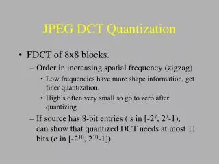
1. JPEG DCT Quantization • FDCT of 8x8 blocks. • Order in increasing spatial frequency (zigzag) • Low frequencies have more shape information, get finer quantization. • High’s often very small so go to zero after quantizing • If source has 8-bit entries ( s in [-27, 27-1), can show that quantized DCT needs at most 11 bits (c in [-210, 210-1])

2. JPEG DCT Quantization • Q(u,v) 8x8 table of integers [1..255] • FQ(u,v) = Round(F(u,v)/Q(u,v)) • Note can have one quantizer table for each image component. If not monochrome image, typically have usual one luminance, 2 chromatic channels. • Quantization tables can be in file or reference to standard • Standard quantizer based on JND. • See Wallace p 12.

3. JPEG DCT IntermediateEntropy Coding • Variable length code (Huffman): • High occurrence symbols coded with fewer bits • Intermediate code: symbol pairs • symbol-1 chosen from table of symbols si,j • i is run length of zeros preceding quantized dct amplitude, • j is length of huffman coding of the dct amplitude • i = 0…15, j= 1…10, and s0,0=‘EOB’ s15,0 = ‘ZRL’ • symbol-2: Huffman encoding of dct amplitude • Finally, these 162 symbols are Huffman encoded.

4. JPEG components • Y = 0.299R + 0.587G + 0.114BCb = 0.1687R - 0.3313G + 0.5BCr = 0.5R - 0.4187G - 0.0813B • Optionally subsample Cb, Cr • replace each pixel pair with its average. Not much loss of fidelity. Reduce data by 1/2*1/3+1/2*1/3 = 1/3 • More shape info in achromatic than chromatic components. (Color vision poor at localization).

5. JPEG goodies • Progressive mode - multiple scans, e.g. increasing spatial frequency so decoding gives shapes then detail • Hierarchical encoding - multiple resolutions • Lossless coding mode • JFIF: • User embedded data • more than 3 components possible?

6. 0 1 10 00s1 01s2 11s3 100s4 101 1010s5 1011s6 Huffman Encoding 1110101101100Traverse from root to leaf, then repeat: 11 1010 11 01 100s3 s5 s3 s2 s4

7. MPEG • MPEG is to temporal compression as JPEG is to static compression: • utilizes known temporal psychophysics, both visual and audio • utilizes temporal redundancy for inter-frame coding (most of a picture doesn’t change very fast)

8. MPEG Data Organization • Inter-frame differences within small blocks: • code difference; good if not much motion • code motion vector; good if translation • Three kinds of frames: • I (Intra); “still” or reference frame, e.g JPEG • P (Predictive) coded relative to I or previous P • B (Bidirectional) coded relative to both previous and next I or P

9. MPEG Data Organization • Goals of inter-frame coding: • high bit rate • random access • Costs • memory • but memory is now cheap, hence HDTV arriving

10. Color TV • Multiple standards - US, 2 in Europe, HDTV standards, Digital HDTV , Japanese analog. • US: 525 lines (US HDTV is digital, and data stream defines resolution. Typically MPEG encoded to provide 1088 lines of which 1080 are displayed)

11. NTSC Analog Color TV • 525 lines/frame • Interlaced to reduce bandwidth • small interframe changes help • Primary chromaticities:

12. NTSC Analog Color TV • These yield 1.909 -0.985 0.058RGB2XYZ = -0.532 1.997 -0.119 -0.288 -0.028 0.902 Y=0.299R + 0.587G +0.114B (same as luminance channel for JPEG!) = Y value of white point. Cr = R-Y, Cb = B-Y with chromaticity: Cr: x=1.070, y=0; Cb: x=0.131 y=0; y(C)=0 => Y(C)=0 => achromatic

13. NTSC Analog Color TV • Signals are gamma corrected under assumption of dim surround viewing conditions (high saturation). • Y, Cr, Cb signals (EY, Er, Eb) are sent per scan line; NTSC, SECAM, PAL do this in differing clever ways EY typically with twice the bandwidth of Er, Eb

14. NTSC Analog Color TV • Y, Cr, Cb signals (EY, Er, Eb) are sent per scan line; NTSC, SECAM, PAL do this in differing clever ways. • EY with 4-10 x bandwidth of Er, Eb • “Blue saving”

15. Digital HDTV • 1987 - FCC seeks proposals for advanced tv • Broadcast industry wants analog, 2x lines of NTSC for compatibility • Computer industry wanta digital • 1993 (February) DHDTV demonstrated • in four incompatible systems • 1993 (May) Grand Alliance formed

16. Digital HDTV • 1996 (Dec 26) FCC accepts Grand Alliance Proposal of the Advanced Televisions Systems Committee ATSC • 1999 first DHDTV broadcasts

17. Digital HDTV lines hpix aspect frames frame rate ratio 720 1280 16/9 progressive 24, 30 or 60 1080 1920 16/9 interlaced 60 1080 1920 16/9 progressive 24, 30 • MPEG video compression • Dolby AC-3 audio compression

18. SWOP ENCAD GA ink Some gamuts

19. Color naming • A Computational model of Color Perception and Color Naming, Johann Lammens, Buffalo CS Ph.D. dissertation http://www.cs.buffalo.edu/pub/colornaming/diss/diss.html • Cross language study of Berlin and Kay, 1969 • “Basic colors”

20. Color naming • “Basic colors” • Meaning not predicted from parts (e.g. blue, yellow, but not bluish) • not subsumed in another color category, (e.g. red but not crimson or scarlet) • can apply to any object (e.g. brown but not blond) • highly meaningful across informants (red but not chartruese)

21. Color naming • “Basic colors” • Vary with language

22. Color naming • Berlin and Kay experiment: • Elicit all basic color terms from 329 Munsell chips (40 equally spaced hues x 8 values plus 9 neutral hues • Find best representative • Find boundaries of that term

23. Color naming • Berlin and Kay experiment: • Representative (“focus” constant across lang’s) • Boundaries vary even across subjects and trials • Lammens fits a linear+sigmoid model to each of R-B B-Y and Brightness data from macaque monkey LGN data of DeValois et. al.(1966) to get a color model. As usual this is two chromatic and one achromatic

24. Color naming • To account for boundaries Lammens used standard statistical pattern recognition with the feature set determined by the coordinates in his color space defined by macaque LGN opponent responses. • Has some theoretical but no(?) experimental justification for the model.