Quantization
Quantization. F(u, v) represents a DCT coefficient, Q(u, v) is a “quantization matrix” entry, and represents the quantized DCT coefficients which JPEG will use in the succeeding entropy coding quantization step is the main source for loss in JPEG

Quantization
E N D
Presentation Transcript
Quantization • F(u, v) represents a DCT coefficient, Q(u, v) is a “quantization matrix” entry, and represents the quantized DCT coefficients which JPEG will use in the succeeding entropy coding • quantization step is the main source for loss in JPEG • The entries of Q(u, v) tend to have larger values towards the lower right corner. This aims to introduce more loss at the higher spatial frequencies — a practice supported by Observations 1 and 2 • default Q(u, v) values obtained from psychophysical studies with the goal of maximizing the compression ratio while minimizing perceptual losses in JPEG images.
The Luminance Quantization Table • The Chrominance Quantization Table 16 11 10 16 24 40 51 61 12 12 14 19 26 58 60 55 14 13 16 24 40 57 69 56 14 17 22 29 51 87 80 62 18 22 37 56 68 109 103 77 24 35 55 64 81 104 113 92 49 64 78 87 103 121 120 101 72 92 95 98 112 100 103 99 17 18 24 47 99 99 99 99 18 21 26 66 99 99 99 99 24 26 56 99 99 99 99 99 47 66 99 99 99 99 99 99 99 99 99 99 99 99 99 99 99 99 99 99 99 99 99 99 99 99 99 99 99 99 99 99 99 99 99 99 99 99 99 99
515 65 -12 4 1 2 -8 5 -16 3 2 0 0 -11 -2 3 -12 6 11 -1 3 0 1 -2 -8 3 -4 2 -2 -3 -5 -2 0 -2 7 -5 4 0 -1 -4 0 -3 -1 0 4 1 -1 0 3 -2 -3 3 3 -1 -1 3 -2 5 -2 4 -2 2 -3 0 F(u, v)
Run-length Coding on AC coefficients • To make it most likely to hit a long run of zeros: a zig-zag scan is used to turn the 8×8 matrix into a 64-vector
DPCM on DC coefficients • The DC coefficients are coded separately from the AC ones. Differential Pulse Code modulation (DPCM)is the coding method • If the DC coefficients for the first 5 image blocks are 150, 155, 149, 152, 144, then the DPCM would produce 150, 5, -6, 3, -8, assuming di = DCi+1 − DCi, and d0 = DC0 • AC components are Huffman coded
Four Commonly Used JPEG Modes • Sequential Mode — the default JPEG mode, each graylevel image or color image component is encoded in a single left-to-right, top-to-bottom scan • Progressive Mode • Hierarchical Mode • Lossless Mode — discussed in Chapter 7
Progressive Mode • Progressive JPEG delivers low quality versions of the image quickly, followed by higher quality passes • Spectral selection: Takes advantage of the “spectral” (spatial frequency spectrum) characteristics of the DCT coefficients: higher AC components provide detail information • Scan 1: Encode DC and first few AC components, e.g., AC1, AC2 • Scan 2: Encode a few more AC components, e.g., AC3, AC4, AC5 • ... • Scan k: Encode the last few ACs, e.g., AC61, AC62, AC63.
Progressive Mode (Cont’d) • 2. Successive approximation: Instead of gradually encoding spectral bands, all DCT coefficients are encoded simultaneously but with their most significant bits (MSBs) first • Scan 1: Encode the first few MSBs, e.g., Bits 7, 6, 5, 4. • Scan 2: Encode a few more less significant bits, e.g., Bit 3. • ... • Scan m: Encode the least significant bit (LSB), Bit 0.
Chapter 10: Video compression • Video consists of a group of frames • An obvious solution to video compression would be predictive coding based on previous frames • Compression proceeds by subtracting images: subtract in time order and code the residual error. • We can do better. Usually the changes are small (high frame rate), and predictable (camera operations such as zoom and pan as well as motion of objects inside the frame) • Scene changes might mean that the frame is similar to its successor than predecessor
Video compression • Video compression using Motion Compensation (MC): • Motion Estimation (motion vector search) • MC-based Prediction • Derivation of the prediction error, i.e., the difference.
Macroblocks and Motion Vector • MV search is usually limited to a small immediate neighborhood — both horizontal and vertical displacements in the range [−p, p]. • This makes a search window of size (2p + 1) x (2p + 1).
10.3 Search for Motion Vectors • Macroblock based (rather than pixel based or object based (MPEG-4). The goal is to find vector that maps block between reference and target frame • The difference between two macroblocks measured by their Mean Absolute Difference (MAD): N—size of the macroblock, kandl — indices for pixels in the macroblock, iandj— horizontal and vertical displacements, C ( x + k, y + l ) — pixels in macroblock in Target frame, R ( x + i + k, y + j + l ) — pixels in macroblock in Reference frame. • The goal of the search is to find a vector (i, j) as the motion vector MV = (u, v), such that MAD(i, j) is minimum:
Sequential Search • Sequential search: sequentially search the whole (2p+ 1) x (2+ 1) window in the Reference frame (referred to as Full search) • a macroblock centered at each of the positions within the window is compared to the macroblock in the Target frame pixel by pixel and their respective MAD • The vector (i, j) that offers the least MADis designated as the MV (u, v) for the macroblock in the Target frame • sequential search method is very costly — assuming each pixel comparison requires three operations (subtraction, absolute value, addition), the cost for obtaining a motion vector for a single macroblock is O ( p2 N2 )
2D Logarithmic Search • Logarithmic search: a cheaper version, that is suboptimal but still usually effective • The procedure for 2D Logarithmic Search of motion vectors takes several iterations and is akin to a binary search: • initially only nine locations in the search window are used as seeds for a MAD-based search; they are marked as ‘1’ • - After the one that yields the minimum MAD is located, the center of the new search region is moved to it and the step-size (“offset”) is reduced to half • - In the next iteration, the nine new locations are marked as ‘2’ and so on
Hierarchical Search • The search can benefit from a hierarchical (multiresolution) approach in which initial estimation of the motion vector can be obtained from images with a significantly reduced resolution. • a three-level hierarchical search in which the original image is at Level 0, images at Levels 1 and 2 are obtained by down-sampling from the previous levels by a factor of 2, and the initial search is conducted at Level 2 • Since the size of the macroblock is smaller and p can also be proportionally reduced, the number of operations required is greatly reduced