Quantization
Quantization. Heejune AHN Embedded Communications Laboratory Seoul National Univ. of Technology Fall 2013 Last updated 2013. 9. 24. Outline . Quantization Concept Quantizer Design Quantizer in Video Coding Vector Quantizer Rate-distortion optimization Concept Lagrangian Method

Quantization
E N D
Presentation Transcript
Quantization Heejune AHN Embedded Communications Laboratory Seoul National Univ. of Technology Fall 2013 Last updated 2013. 9. 24
Outline • Quantization Concept • Quantizer Design • Quantizer in Video Coding • Vector Quantizer • Rate-distortion optimization Concept • Lagrangian Method • Appendix • Detail for Lloyd-max Quantization Algorithm
1. Quantization • Reduce representation set • Nlarge points ([0 ~ Nlarge]) to Nsmall points ([0, … Nsmall]) • Inevitable when Analog to Digital Conversion • Not Reversible ! ReScale ADC/Quant Original (digital/analog) Quanitzed Levels
Scalar Quantizer Q q • Quantize a single value (single input & single output) • In contrast to VQ (Vector Quantizer, to be discussed later) • Mapping function • {[xi-1, xi) => yi} • Decision levels to reconstruction level -1 Q q Quantizer output yi Output : {yi} xi-1 xi Quantizer input Input : x
Quantizer’s Effects • + Bit Rate Reduction • Bits required to represent the values: (E1bits=> E2 bits) • Nlarge (= 2E1)points ([0 ~ N]) to Nsmall (= 2E2)points ([0, … Nsmall]) • Bit reduction = E2 - E1 = log2 (NLarge/Nsmall) • - Distortion • e = yi - x (in [xi-1, xi)) • MSE (mean squared error) • Trade-off problem
2. Quantization Design • Distortion • Quantization error = difference original (x) and quantized (yi) • Distortion Measure • Quantizer design parameters • Step size (N) • decision level (xi) • reconstruction level (yi) • Distortion depends on Input signal distribution (f(x)) • Optimization Problem • How to set the ranges and reconstruction values, i.e., {yi & [xi-1, xi)} for i =0, … N, so that the resulting MSE is minimized.
Optimal Quantizer • Solutions • Note performance depends on the input statistics. • Simpler design • Uniform (Fixed quant step) quantizer • With/Without dead-zone near zero • Lloyd-Max algorithm • a optimal quantizer design algorithm • More levels for dense region, Less levels for sparse region. (non-linear quantizer)
Uniform Midrise Quantizer Uniform Midtread Quantizer Reconstruction Reconstruction 3.5∆ 3∆ 2.5∆ 2∆ 1.5∆ ∆ 0.5 ∆ -3∆ -2∆ -∆ -2.5∆ -1.5∆ -0.5∆ -0.5∆ ∆ 2∆ 3∆ Input 0.5∆ 1.5∆ 2.5∆ Input -∆ -1.5∆ -2∆ -2.5∆ -3∆ -3.5∆ Uniform Quantizers • Properties • xi and yi are spaced evenly (so, uniform), with space Δ (step size) • Mid-tread (odd # of recon. levels) vs Mid-rise (no zero recon. ) • mid-tread is more popular than mid-rise. What will be the mathematical representation for quant/inverse?
Uniform Quantizer Performance • For Uniform dist. Input, Uniform quantizer is optimal • Can you prove this? • Uniform Input X ~ U(-A,A) • Error signal e = y – x ~ U(-Δ/2, Δ/2)
Signal Power (variance) • MSE • SNR • Note • If one bit added, Δ is halved, noise variance reduces to 1/4, SNR increases by 6 dB. • SNR does not depends on input range, MSE does.
Non-uniform Quantizer • Issue • Many data are non-uniformly distributed and even unbounded • Concept • General Intuition: Dense Levels for Dense Input region • Boundness: Use saturation Post filter for unbounded input • Generally no closed-form expression for MSE. • Range and Reconstruction Level is cross-related
Lloyd-Max Algorithm • Algorithm • Iteration algorithm with decision level (xi) and recon. level (yi) • Run until code book does not change any more • Step 1: find Near Region Ri((xi-1 , xi]) • Ri = {x | d(x,yi) <= d(x,yj), for all j =\= I } • Step 2: find level yi • yi = E[X| x in Ri ] centroid calculation range update
Lloyd-Max Algorithm • Minimize mean squared error. where Tk is the k th interval [tk,tk+1)
Example • Quantization and Quality (Lloyd-Max applied) • Original (8bpp) vs 6 bpp (spatial domain)
High Density Quantization • High Quality • Condition • Observation • Slow change (Constant) over the quantization region • Approximate with Uniform distribution conditional pdf of in the interval
Quantization in Video Coding • UTQ (uniform Threshold Quantization) often is used • Difficult in adaptive design (a LM quantizer design) • Video quantizers are high quality ones • Quantization in VC • Input signal: quantize the (DCT) coefficients • Parameters • q (Δ): quantization scale factor ( 2 ~ 62, usu. q = 2QUANT, 1 ~31 ) • Index (Level) : index for the reconstruction values • Note: index, not reconstruction values are transmitted • E.g. • Index: I (n,m) = floor(F(n,m)/q) = floor(F(n,m)/2QUANT) • i.e. [i-1, i) *q => i • Reconstruction: F’(n.m) = (I(n,m) + ½) x q = (2*I(n,m) +1)xQUANT • i.e. i => (i +1/2) q (i.e, middle of range [i -1, i)*q) • Note: with QUANT, no 1/2 in expression.
Uniform Threshold Quantizer • Threshold (dead zone) for reducing dct coeff. • Intra DC (zero threshold), Intra AC, inter DC, AC (non-zero) • 2*Q(UANT) = q AC (With Threshold) DC (without Threshold, q = 8 ) Quantizer Quantizer output output 3q 5Q 2q 3Q q q -q -3Q dead zone -2q -3q -q/2 -5Q q -2Q 2Q Quantizer 3q 5Q Quantizer q/2 2q 3Q input -q -Q input -2q -3Q -3q -5Q
3. Quantization in Video Coding • Applied on the Transform Coefficients • Key Throttle for Bit-Rate and Quality • Very Important Trade-off in Video coding Estimation (MC, IntraP) Transform (e.g. DCT) Quantization Entrophy Coding Xorig e = Xorig - Xest Yq = Q(Y) VLC(Yq) Y = T(e)
Example #1 • Example #2: Comparison with Coarse and Fine Quant • See Textbook Table 7.4 Q(8) Transformed 8x8 block Zig-zag scan
DCT Coef. Quantization • Human visual weight • coarse quant to High frequency components • NDZ-UTQ to Intra DC, DZ-UTQ to all others • Intra block Case • I (n,m) = round(F(n,m)/(q*W(n,n))/8 ) • F’(n.m) = (I(n,m) + ½) x q x W(n,m)/8
31 34 27 27 26 23 19 19 18 15 11 11 10 7 3 0 0 Len = 14 > 8 Len = 14 > 8 -7 -10 -11 -11 -15 -18 -19 -19 -23 -26 -27 -27 -31 -34 Quantizer Example • MPEG-4 example • Inverse Quantization only Defined if LEVEL = 0, REC = 0 Else If QUANT is ODD |REC| = QUANT *(2 |LEVEL| +1) Else |REC| = QUANT *(2|LEVEL| +1) -1 • + 1 : Dead-zone • (sorry, I cannot explain why odd/even) • Quantization is not defined • Why? • Examples • Q= 4 Un-biased biased
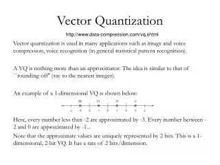
4. Vector Quantizater • Vector Quantizer • Use statistical correlation of N dimension Input
Vector Quantizer Design Generalized Loyd-Max Algorithm Why Not Vector Quantization in Video Standards Transform Coding utilizes the “Correlation”, the remaining signal does not has Correlation much.
Embedded quantizers • Motivation: “scalability” – decoding of compressed bitstreams at different rates (with different qualities) • Nested quantization intervals • In general, only one quantizer can be optimum(exception: uniform quantizers) x Q0 Q1 Q2
Rate Distortion Theory • Rate vs Distortion • Inverse relation between Information/Data Rate and Distortion • Revisit to a uniform distributed r.v. with a uniform quantizer • Plot it ! Exponential decreasing Proportional to Complexity of source in statistics
Rate Distortion Theory • Rate-distortion Function and Theroy • Inverse relation between Information/Data Rate and Distortion • Example with Gaussian R.V.
Rate-Distortion Optimization • Motivation • Image coding • Condition: we can use 10KBytes for a whole picture • Each part has different complexity (i.e, simpler and complex, variance) • Which parts I have to assign more bits? • Analogy to school score • Students are evaluated sum of Math and English grade. • I gets 90pts in Math, 50pts in Eng. • Which subject I have to study? • (natural assumption: 90 to 100 is much harder than 50 to 60) simpler blocks More complex blocks
Lagrange multiplier • Constrained Optimization Problem • Minimize distortion with bits no larger than max bits • Cannot use partial differential for minima and maxima • Lagrange Multiplier technique • Insert one more imaginary variable (called Lagrange) • We have multivariable minimization problem
1 1 Side note: why not partial differential • Simple example • min subject to • Solution • By substitution • minimum ½ at x = y = 1/sqrt(2) • Wrong Solution • With complex constraints, we cannot use substitution of variable method • We cannot change partial different with ordinary difference • If we check, • x = y = 0 ?
An Example: Lagrange Multiplier • Optimization Problem • multiple independent Gaussian variables • Lagrange multiplier optimization
Solution • Multiplying M equations, and take M-square • Lagrange value • Bit-allocation • Large variance, then more bit allocation • But the increment is logarithmic (not linear)
Appendix Lloyd-Max Algorithm Details
Lloyd-Max scalar quantizer • Problem : For a signal x with given PDF find a quantizer with M representative levels such that • Solution : Lloyd-Max quantizer [Lloyd,1957] [Max,1960] • M-1 decision thresholds exactly half-way between representative levels. • Mrepresentative levels in the centroid of the PDF between two successive decision thresholds. • Necessary (but not sufficient) conditions
Iterative Lloyd-Max quantizer design • Guess initial set of representative levels • Calculate decision thresholds • Calculate new representative levels • Repeat 2. and 3. until no further distortion reduction
Boundary Reconstruction Example of use of the Lloyd algorithm (I) • X zero-mean, unit-variance Gaussian r.v. • Design scalar quantizer with 4 quantization indices with minimum expected distortion D* • Optimum quantizer, obtained with the Lloyd algorithm • Decision thresholds -0.98, 0, 0.98 • Representative levels –1.51, -0.45, 0.45, 1.51 • D*=0.12=9.30 dB
Example of use of the Lloyd algorithm (II) • Convergence • Initial quantizer A:decision thresholds –3, 0 3 • Initial quantizer B:decision thresholds –½, 0, ½ • After 6 iterations, in both cases, (D-D*)/D*<1%
Threshold Representative Example of use of the Lloyd algorithm (III) • X zero-mean, unit-variance Laplacian r.v. • Design scalar quantizer with 4 quantization indices with minimum expected distortion D* • Optimum quantizer, obtained with the Lloyd algorithm • Decision thresholds -1.13, 0, 1.13 • Representative levels -1.83, -0.42, 0.42, 1.83 • D*=0.18=7.54 dB
Example of use of the Lloyd algorithm (IV) • Convergence • Initial quantizer A, decision thresholds –3, 0 3 • Initial quantizer B,decision thresholds –½, 0, ½ • After 6 iterations, in both cases, (D-D*)/D*<1%
Lloyd algorithm with training data • Guess initial set of representative levels • Assign each sample xi in training set T to closest representative • Calculate new representative levels • Repeat 2. and 3. until no further distortion reduction
Lloyd-Max quantizer properties • Zero-mean quantization error • Quantization error and reconstruction decorrelated • Variance subtraction property