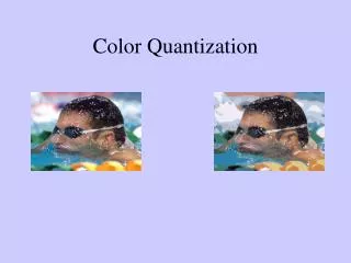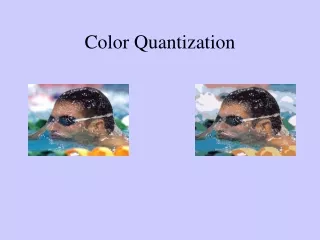
Quantization results
Quantization results. Observations leading to MacAdam Ellipses. Weber’s Law of “Just Noticeable Difference” (difference threshold).


Quantization results
E N D
Presentation Transcript
Observations leading to MacAdam Ellipses Weber’s Law of “Just Noticeable Difference” (difference threshold) Ernst Weber, a 19th century experimental psychologist, observed that the size of the difference threshold appeared to be lawfully related to initial stimulus magnitude. This relationship, known since as Weber's Law, can be expressed as: (Ex: weight lifting)
Typical Log curve sensitivity white dark OBSERVATIONS (contd.) • Distances measured in RGB space do not relate to human perception of color differences. • Fechner’s Law: We are more sensitive to changes in darker regions than in lighter regions.(ex:Log. response from dark(0) to white(255)) • Perceived Sensation S = k log(I) , where I is Stimulus
OBSERVATIONS (contd.) • We are more sensitive to intensity changes than the hue shifts. • Perceptual versus Linear (mathematical) quantization. • Quantization errors are spatially and temporally (ex: illumination) dependent
OBSERVATIONS (contd.) • We are more sensitive to errors at lower spatial frequencies (ex: uniform region, or a low sound in a quiet place). Sensitivity Spatial frequency 1 30
Two sources radiating different spectral distributions may or may not appear to be the same color for the average human observer. However, their color specifications will be different. Chromaticity,ie. quality of color, is specified by a point in the Tongue. • Similarly, colors of reflecting materials are specified. Several samples, having different spectral reflectance characteristics, appear alike under certain conditions of illumination. • These specifications give precise meaning to color standards, in quantitative values which are reproducible.
MacAdam Ellipses “Visual sensitivities to color differences in Daylight” by David L. MacAdam, Journ.Optical Soc. of America, May 1942,Vol. 32,pp247-274. • Pairs of variable colors are presented (No variation of luminance). • A criterion of visual sensitivity to color difference-- the standard deviation of color matching-- was studied as a reproducible criterion. The chromaticity of illumination was an average “Daylight”. The experiment is described in this paper. • Over 2500 trials of color matching were observed for a single observer. The standard deviations of trials are represented in terms of distance (line segments) in the Standard Chromaticity diagram (Tongue). The directions correspond to departures from points representing std. chromaticities.
MacAdam • Small, equally noticeable chromaticity differences are represented for all chromaticities and for all kinds of variations by the lengths of radii of a family of ellipses i.e. the end of each radius corresponds to noticeable color difference. • All visual stimuli are produced by additive mixtures of filtered beams from a single calibrated light source.
Standard Deviations of Color Matching • Several criteria were investigated for the measurement of the noticeability of color differences. • The Just Noticeable Difference (JND) was used extensively.
MacAdam Ellipses for color Quantization (sumanth, CB, BLD) • Since an ellipse in the CIE xy diagram represents a color, and since RGB space is a subset of this, it should be possible to fill the displayable RGB color space (in the Tongue diagram) with ellipses. • Instead of conducting experiments, the 25 McAdam ellipses are used with linear interpolation.
Every color point can be divided into luminance (Y) part and chromaticity (x, y). • We know color discrimination improves under stronger illumination. Human eye is sensitive to luminance compared to chromaticity. • Therefore, we prefer more levels in Luminance compared to Chromaticity. • There exits tradeoff between Luminance and Chromaticity, since the total quantization steps are equal to the number of levels of quantization in both the above.
To recollect Intensity • Intensity is a measure over some interval of the electromagnetic spectrum of the flow of power that is radiated from, or incident on, a surface. Intensity is what we call a linear-light measure, expressed in units such as watts per square meter. • The voltages presented to a CRT monitor control the intensities of the color components, but in a nonlinear manner. CRT voltages are not proportional to intensity.
To recollect luminance • Brightness is defined by the CIE as the attribute of a visual sensation according to which an area appears to emit more or less light . Because brightness perception is very complex, the CIE defined a more tractable quantity luminance which is radiant power weighted by a spectral sensitivity function that is characteristic of vision.
To recollect Photopic Spectral Sensitivity Function This graph is an illustration of the relative photopic spectral sensitivity for human vision. Humans are most sensitive at the middle wavelengths and their spectral sensitivity falls off towards the long and short wavelengths.
To recollect luminance • Luminance is a photometric measure of the luminous intensity per unit area of light traveling in a given direction. It describes the amount of light that passes through or is emitted from a particular area, and falls within a given solid angle. The SI unit for luminance is candela per square metre (cd/m2). The CGS unit of luminance is the stilb, which is equal to one candela per square centimeter or 10 kcd/m2 • Luminance is defined by • where • Lv is the luminance (cd/m2), • F is the luminous flux or luminous power (lm), • is the angle between the surface normal and the specified direction, • A is the area of the surface (m2), and • is the solid angle (sr).
This research paper work involves: • Linear interpolation of McAdam ellipses • Application to color quantization • Comparison with median cut and octree approaches.
Experiments on MacAdam Ellipses • All the 25 MacAdam ellipses were plotted in the x-y CIE chromaticity space. Each ellipse is characterized by five parameters, which include ‘a’ length of semi major axis, ‘b’ length of semi minor axis, ‘x0’ x-coordinate of its center, ‘y0’ y-coordinate of its center and ‘theta’(degrees) the orientation of the major axis with respect to the horizontal. Collected these parameters from his original data on graph sheet. The 25 ellipses have been reconstructed using the mathematical equations below: • x = x0 (j) + a (j) cos (theta (j)) pi/180) cos (t) - b (j) sin (theta (j)) pi/180) sin (t); • y = y0 (j) + a (j) sin (theta (j)) pi/180) cos (t) + b (j) cos (theta (j)) pi/180) sin (t); • J=ellipse number, t is a parameter for an ellipse • Plot of these ellipses is shown in fig 1.
Plot of these ellipses when transformed into the RGB space (cube), produced ellipses which all lie on a plane for a constant value of illumination (Y). A general property of RGB color space is that for a constant value of illumination all the set of RGB colors lie in a plane (Y = 0.2125R + 0.7154G + 0.0721B) in the RGB color space. Fig 1. x,y – CIE chromaticity space: The ellipses are enlarged 5 times their size with the RGB triangle superimposed:
Experiment • The experiment involves plotting the selected 8 neighboring color points around a test color point. These neighboring points are obtained by a process of interpolating MacAdam ellipses. • To verify this experiment, a MacAdam ellipse is chosen.
Experiment I: • First experiment included plotting of nine color points of a MacAdam ellipse with center coordinates as (0.305, 0.3225), which included the center of the ellipse, four points lying on the boundary of the ellipse, mid points of these boundary points and the center. • These nine colors were displayed and found that they are indistinguishable as observed by 3 observers. For further investigation, a point outside the ellipse was taken and found to be distinguishable when compared with the center color point of the ellipse as observed by the same 3 observers. This established the consistency within an ellipse.
Fig 2(a) C: Center of the ellipse 1 – 8 are color points of the ellipse as shown in fig 2(b) Fig 2. (Colors arranged as per fig 2(a)) Fig 2(b)
Experiment II: • Consider the CIE x,y chromaticity space. Consider a test color point in this x,y space. we propose an algorithm of linear interpolation of the 25 MacAdam ellipses which will compute the ellipse around the given test color point with center of the ellipse as the test color point. • The interpolation being linear, assumes that any parameter of an ellipse is inversely proportional to the distance from the centers of these 25 MacAdam ellipses.
Experiment II has been performed at the same point (0.305,0.3225) as the center of the ellipse and the results are shown in fig 3. When observed by the same 3 observers, all the 9 color points as displayed in fig 3 appeared the same. This expt. Proved again the consistency by taking a point within an ellipse ,obtained by interpolation. Fig 3 colors arranged as per fig 2(a)
Some experiments are done to increase the accuracy of the interpolated results. Out of 5 parameters of an ellipse, two are known x0 and y0. • We need to interpolate 3 unknown parameters to generate the ellipse around the test color point. The ellipse around the test color point is generated by 3 approaches. • Linear interpolation of the 3 unknown parameters of the desired ellipse, using the 25 MacAdam ellipses. At the chosen center point of the ellipse (0.305 , 0.3225) , this approach resulted in an ellipse as shown by curve 4 in fig 4.This approach cannot give good results, since the ellipses are spread out nonlinearly. 2. Linear interpolation of 3 unknown parameters of the desired ellipse using the two nearest ellipses. The resulting ellipse interpolated for (0.305, 0.3225) as test color point, is shown in Fig 4 as curve 2. (Contd..)
3.Here we assume that any ellipse is a point in the five dimensional space with 5 dimensions being the 5 parameters of the ellipse. Now we interpolate for the 3 unknown parameters of the ellipse using the 25 points in the 5 dimensional space corresponding to the 25 MacAdam ellipses in the x,y chromaticity space. The resulting ellipse interpolated for (0.305, 0.3225) as test color point, is as shown in Fig 4 curve 3 while the curve 1 in fig 4 corresponds to the original MacAdam ellipse at (0.305, 0.3225). Fig. 4
III Application to color quantization: • If the CIE x,y chromaticity space is made up of MacAdam ellipses, would give rise to a method of quantizing the entire color space into as many distinguishable colors as perceived. Using the concept of MacAdam ellipses, we can estimate the number of distinguishable colors that fall in the RGB space. This number would be nearly the total area of the RGB triangle divided by the average area of the 25 MacAdam ellipses. Area of the RGB triangle with vertices (0.15, 0.06), (0.3, 0.59) and (0.63, 0.33) is 0.1069 sq units. Average area of 25 ellipses is 0.000014 sq units. The number of distinguishable colors in RGB triangle would be thus 0.1069/ 0.000014 which is 7636. This number is almost in the agreement with the literature figures for color discrimination by humans.
III Application to color quantization: (Contd..) • Color can be divided into two parts: the luminance (Y) and the chromaticity coordinates (x, y). Quantization of color would be quantization of luminance as well as chromaticity. Suppose we want to quantize the colors in an image into 64 colors, then we can quantize Y into 4 levels and quantize chromaticity into 16 levels or vice versa. So there appears to be a trade off between luminance and chromaticity in the process of quantization. We would explicitly explain the importance of luminance over the chromaticity through results obtained from the two-quantization algorithms that we are proposing here.
quantization of chromaticity: • The CIE x,y chromaticity space consists of various points (x,y) each one of which represents a different color. quantization of chromaticity (in the RGB triangle) would mean selecting certain number of these points (x, y). These selected chromaticity points may also be called as seed points. In this algorithm we are fixing these seed points in the process of quantization of chromaticity. We have done experiments for 4 as well as 16 levels of quantization in chromaticity. quantization of chromaticity into K levels means fixing K seed points in the RGB color triangle. This can be achieved by dividing the RGB triangle into K equal triangles, and circum- centers of these K triangles will give us K seed points. For example to get 4 seed points, the RGB triangle is divided into 4 triangles. This can be achieved by joining the mid points of the sides of RGB triangle (see Fig 5(a)). In a similar way for 16 seed points each one of these 4 triangles have to be further divided into 4 triangles each and the circum-centers of these 16 triangles will gives us 16 seed points as given in Fig 5 (b).
G B R Fig 5(a) - Four levels Fig 5 (b) – Sixteen levels
Fig 6 (a) Fig 6 (b) ( 4 x 8) Fig 6 (c) ( 4 x 16) Fig 6 (d) ( 4 x 32) Fig 6 (e) ( 8 x 4) Fig 6 (f) (8 x 8 ) (chromaticity levels x luminance levels)
Fig 6 (g) (8 x 16) Fig 6 (h) ( 8 x 32) Fig 6 (i) ( 16 x 4) Fig 6 (j) ( 16 x 8) Fig 6 (k) ( 16 x 16) Fig 6 (l) (32 x 4)
Fig 6 (m) ( 32 x 8) Lena originally has very few colors, therefore greater quantization in chrominance leads to no improvement.
Fig 7 (a) Fig 7 (b) ( 4 x 8 ) Fig 7 (c) ( 4 x 16 ) Fig 7 (d) ( 4 x 32 ) Fig 7 (e) ( 8 x 4 ) Fig 7 (f) ( 8 x 8 ) (chromaticity levels x luminance levels)
Fig 7 (g) ( 8 x 16 ) Fig 7 (h) ( 8 x 32 ) Fig 7 (i) ( 16 x 4) Fig 7 (m) ( 32 x 8 ) Fig 7 (j) ( 16 x 8) Fig 7 (k) ( 16 x 16) Fig 7 (l) (32 x 4 ) Mandrill has many colors and not much variation in brightness. Therefore, increasing quantization in Chrominance improves image quality.
Quantization Algorithm II:A different approach for quantizing chromaticity Quantization of chromaticity: In this algorithm for quantization, instead of pre-fixing the chromaticity seed points, we would select these chromaticity points based on the input image. Thus this algorithm becomes adaptive unlike the quantization algorithm 1. Suppose we want to quantize the chromaticity into k levels, then we would be required to choose k chromaticity points from the RGB color space. • These k points are chosen in an adaptive way as described below. We apply a k-means clustering algorithm to divide the entire image into k clusters and then the mean point of each of the clusters becomes the seed point for quantization of chromaticity space. In the quantization algorithm I, these k seed points were fixed and in this algorithm these seed points are dependent on the input image. The results obtained by implementing this algorithm are given in Fig 8 and Fig 9.
(chromaticity levels x luminance levels) Fig 8 (a) Fig 8 (b) ( 4 x 8 ) Fig 8 (c) ( 4 x 16 ) Fig 8 (d) ( 4 x 32 ) Fig 8 (e) ( 8 x 4 ) Fig 8 (f) ( 8 x 8)
Fig 8 (g) ( 8 x 16 ) Fig 8 (h) ( 8 x 32 ) Fig 8 (i) ( 16 x 4 ) Fig 8 (j) ( 16 x 8) Fig 8 (k) ( 16 x 16) Fig 8 (l) (32 x 4 ) Fig 8 (m) ( 32 x 8 ) No odd colors appeared in this method.
Fig 9 (a) Fig 9 (b) ( 4 x 8 ) Fig 9 (c) ( 4 x 16 ) Fig 7(f) (8x8) For comparison Fig 9 (d) ( 4 x 32 ) Fig 9 (e) ( 8 x 4 ) Fig 9 (f) ( 8 x 8)
Fig 9 (g) ( 8 x 16 ) Fig 9 (h) ( 8 x 32 ) Fig 9 (i) ( 16 x 4 ) Fig 9 (m) ( 32 x 8 ) Fig 9 (j) ( 16 x 8) Fig 9 (k) ( 16 x 16) Fig 9 (l) (32 x 4 )