Scalar Quantization
Scalar Quantization. CAP5015 Fall 2004. Quantization. Definition: Quantization: a process of representing a large – possibly infinite – set of values with a much smaller set. Scalar quantization: a mapping of an input value x into a finite number of output values, y : Q: x ® y


Scalar Quantization
E N D
Presentation Transcript
Scalar Quantization CAP5015 Fall 2004
Quantization • Definition: • Quantization: a process of representing a large – possibly infinite – set of values with a much smaller set. • Scalar quantization: a mapping of an input value x into a finite number of output values, y: Q: x ® y • One of the simplest and most general idea in lossy compression.
Scalar Quantization • Many of the fundamental ideas of quantization and compression are easily introduced in the simple context of scalar quantization. • An example: any real number x can be rounded off to the nearest integer, say q(x) = round(x) • Maps the real line R(a continuous space) into a discrete space.
Quantizer • The design of the quantizer has a significant impact on the amount of compression obtained and loss incurred in a lossy compression scheme. • Quantizer: encoder mapping and decode mapping. • Encoder mapping • – The encoder divides the range of source into a number of intervals • – Each interval is represented by a distinct codeword • Decoder mapping • – For each received codeword, the decoder generates a reconstruct value
Components of a Quantizer • Encoder mapping: Divides the range of values that the source generates into a number of intervals. Each interval is then mapped to a codeword. It is a many-to-one irreversible mapping. The code word only identifies the interval, not the original value. If the source or sample value comes from a analog source, it is called a A/D converter.
Mapping of a 3-bit Encoder Codes … 000 001 010 011 100 101 110 111 -3.0 -2.0 -1.0 0 1.0 2.0 3.0 input
Components of a Quantizer 2. Decoder: Given the code word, the decoder gives a an estimated value that the source might have generated. Usually, it is the midpoint of the interval but a more accurate estimate will depend on the distribution of the values in the interval. In estimating the value, the decoder might generate some errors. (Give Table 8.1 and explain)
Probability Density Function • A probability density function f(x) of the random variable x is said to meet the following criterion : • Probability associated with a value of x in its domain X is given by Pr( X<= x ). • The corresponding cumulative distribution function CDF or F(x) requires that F(x) is non-decreasing for x[1] <= x[2]. When sampling occurs at discrete intervals then F(x) is said to be monotonically increasing. • F(x) is said to be continuous from the right or that the limit of f(x + e) exists when evaluated as e-> 0 from the right positive abscissa. • In the discrete case the point probabilities of particular values of x[i] have a probability that is always greater or equal to 0, p[i] == Pr( X = x[i] ) >= 0. • CDF may be expressed as • In the continuous case, the CDF may be expressed as the following relationship:
Quantization operation: • – Let M be the number of reconstruction levels where the decision boundaries are and the reconstruction levels are
Quantization Problem • MSQE (mean squared quantization error) • If the quantization operation is Q • Suppose the input is modeled by a random variable X with pdf fX(x). The MSQE is
Quantization Problem • Rate of the quantizer • The average number of bits required to represent a single quantizer output • –For fixed-length coding, the rate R is: • For variable-length coding, the rate will depend on the probability of occurrence of the outputs
Quantization Problem • Quantizer design problem • Fixed -length coding • Variable-length coding If li is the length of the codeword corresponding to the output yi, and the probability of occurrence of yi is: The rate is given by:
Uniform Quantizer Zero is one of the output levels M is odd Zero is not one of the output levels M is even
Image Compression Original 8bits/pixel 3bits/pixel
Image Compression 2bits/pixel 1bit/pixel