Uniform Quantization

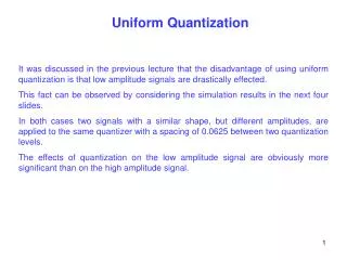
1. Uniform Quantization It was discussed in the previous lecture that the disadvantage of using uniform quantization is that low amplitude signals are drastically effected. This fact can be observed by considering the simulation results in the next four slides. In both cases two signals with a similar shape, but different amplitudes, are applied to the same quantizer with a spacing of 0.0625 between two quantization levels. The effects of quantization on the low amplitude signal are obviously more significant than on the high amplitude signal.

2. Uniform Quantization Max Amplitude = 1 Input Signal 1.

3. Uniform Quantization Quantized Signal 1. Δv=0.0625

4. Max Amplitude = 0.125 Uniform Quantization Input Signal 2.

5. Uniform Quantization Quantized Signal 2. Δv=0.0625

6. Uniform Quantization Figure-1 Input output characteristic of a uniform quantizer.

7. Uniform Quantization Recall that the Signal to Quantization Noise Ratio of a uniform quantizer is given by: This equation verifies the discussion on slide-1 that SNqR for a low amplitude signal is quite low. Therefore, the effect of quantization noise on such audio signals should be noticeable. Lets consider the case of voice signals (see next slide)

8. Uniform Quantization Click on the following links to listen to a sample voice signal. First play “voice file-1”; then play “voice file-1 Quantized”. Do you notice the degradation in voice quality? This degradation can be attributed to uniformly spaced quantization levels. Voice file-1 Voice file-1. Quantized (uniform) Note: You may not notice the difference between the two clips if you are using small laptop speakers. You should use either headphones or larger speakers.

9. Uniform Quantization More insight into signal degradation can be gained by looking at the voice signal’s Histogram. A histogram shows the distribution of values of data. Figure-2 below shows the histogram of the voice signal-1. Most of the values have low amplitude and occur around zero. Therefore, for voice signals uniform quantization will result in signal degradation. Figure-2 Histogram of voice signal-1

10. Non-Uniform Quantization The effect of quantization noise can be reduced by increasing the number of quantization intervals in the low amplitude regions. This means that spacing between the quantization levels should not be uniform. This type of quantization is called “Non-Uniform Quantization”. Input-Output Characteristics shown below.

11. Non-uniform Quantization Non-uniform quantization is achieved by, first passing the input signal through a “compressor”. The output of the compressor is then passed through a uniform quantizer. The combined effect of the compressor and the uniform quantizer is that of a non-uniform quantizer. (see figure 3.) At the receiver the voice signal is restored to its original form by using an expander. This complete process of Compressing and Expanding the signal before and after uniform quantization is called Companding.

12. Non-uniform Quantization (Companding) y=g(x) 1 -1 x=m(t)/mp 1 -1 Input output relationship of a compressor.

13. Non-uniform Quantization (Companding) A-Law (USA) Where, The value of ‘µ’ used with 8-bit quantizers for voice signals is 255

14. Non-uniform Quantization (Companding) The µ-law compressor characteristic curve for different values of ‘µ’.

15. Compressor Uniform Quantizer Expander Non-uniform Quantization (Companding) Click on symbols to listen to voice signal at each stage 15

16. Compressor Uniform Quantizer Expander Non-uniform Quantization (Companding) Click on symbols to listen to voice signal at each stage The 3 stages combine to give the characteristics of a Non-uniform quantizer. 16

17. Uniform Quantizer Non-uniform Quantization (Companding) Click on symbols to listen to voice signal at each stage A uniform quantizer with input and output voice files is presented here for comparison with non-uniform quantizer.

18. Non-Uniform Quantization Lets have a look at the histogram of the compressed voice signal. In contrast to the histogram of the uncompressed signal (figure-2) you can see that the values are now more distributed. Therefore, it can be said that the compressor changes the histogram/ pdf of the voice signal from gaussian (bell shape) to a uniform distribution (shown below). Figure-3 Histogram of compressed voice signal

19. Non-Uniform Quantization Where is the Compression..??? The compression process in Non-uniform quantization demands some elaboration for clarity of concepts. It should be noted that the compression mentioned in previous slides is not the time or frequency domain compression which students are familiar with. This can be verified by looking at the time domain waveforms at the input and output of the compressor. Note that both the signals last for 3.75 seconds. Therefore, there is no compression in time or frequency. Fig-4-a Signal at Compressor Input Fig-4-b Signal at Compressor Output

20. Non-Uniform Quantization Where is the Compression..??? The compression here occurs in the amplitude values. An intuitive way of explaining this compression in amplitudes is to say that the amplitudes of the compressed signal are more closely spaced (compressed) in comparison to the original signal. This can also be observed by looking at the waveform of the compressed signal (fig-4-b). The compressor boosts the small amplitudes by a large amount. However, the large amplitude values receive very small gain and the maximum value remains the same. Therefore, the small values are multiplied by a large gain and are spaced relatively closer to the large amplitude values. A parameter which can be used to measure the degree of compression here is the Dynamic range. “The Dynamic Range is the ratio of maximum and minimum value of a variable quantity such as sound or light” [ ]. In the simulations the Dynamic Range (DR) of the compressor input = 41.45 dB Whereas Dynamic Range (DR) of compressor output = 13.95 dB

21. Reference Text Books • Lecture Notes “Advanced Digital Communications” by Dr. Norbert Goertz. MSc Signal Processing & Communication January 2007, The University of Edinburgh. • “Modern Digital & Analog Communications” 3rd Edition by B. P. Lathi. • “Digital & Analog Communication Systems” 6th Edition by Leon W. Couch, II. • “Communication Systems” 4th Edition by Simon Haykin. • “Analog & Digital Communication Systems” by Martin S. Roden. • Sample voice file taken from CD of Digital Signal Processing a Computer Based Approach By S. K. Mitra. • Note: With the exception of figures on slides 06 and 14 all figures have been sketched by Hassan Aqeel Khan. The voice files have been generated by using Matlab 7. 21