Scalar Visualization
Scalar Visualization. Outline. Visualizing scalar data A number of the most popular scalar visualization techniques Color mapping Contouring Height plots. Color mapping Design of effective colormaps Contouring in 2D and 3D Height plots. Visualization Pipeline. 1. Data Importing

Scalar Visualization
E N D
Presentation Transcript
Outline • Visualizing scalar data • A number of the most popular scalar visualization techniques • Color mapping • Contouring • Height plots • Color mapping • Design of effective colormaps • Contouring in 2D and 3D • Height plots
Visualization Pipeline 1. Data Importing 2. Data Filtering 3. Data Mapping 4. Date Rendering
Color Mapping • color look-up table • Associate a specific color with every scalar value • The geometry of Dv is the same as D
Luminance Colormap • Use grayscale to represent scalar value • Most scientific data (through measurement, observation, or simulation) are intrinsically grayscale, not color Luminance Colormap Legend
Rainbow Colormap • Red: high value; Blue: low value • A commonly used colormap Luminance Map Rainbow Colormap
Rainbow Colormap • Construction • f<dx: R=0, G=0, B=1 • f=2: R=0, G=1, B=1 • f=3: R=0, G=1, B=0 • f=4: R=1, G=1, B=0 • f>6-dx: R=1, G=0, B=0
Rainbow Colormap Implementation void c(float f, float & R, float & G, float &B) { const float dx=0.8 f=(f<0) ? 0: (f>1)? 1 : f //clamp f in [0,1] g=(6-2*dx)*f+dx //scale f to [dx, 6-dx] R=max(0, (3-fabs(g-4)-fabs(g-5))/2); G=max(0,(4-fabs(g-2)-fabs(g-4))/2); B=max(0,(3-fabs(g-1)-fabs(g-2))/2); }
Colormap: Designing Issues • Choose right color map for correct perception • Grayscale: good in most cases • Rainbow: e.g., temperature map • Rainbow + white: e.g., landscape • Blue: sea, lowest • Green: fields • Brown: mountains • White: mountain peaks, highest
Rainbow Colormap http://atmoz.org/img/weatherchannel_national_temps.png
Exp: Earth map http://www.oera.net/How2/PlanetTexs/EarthMap_2500x1250.jpg
Exp: Coronal loop http://media.skyandtelescope.com/images/SPD+on+CME+image+5+--+TRACE.gif
Color Banding Effect Caused by a small number of colors in a look-up table
Contouring • A contour line C is defined as all points p in a dataset D that have the same scalar value, or isovalue s(p)=x • A contour line is also called an isoline • In 3-D dataset, a contour is a 2-D surface, called isosurface
Contouring Cartograph
Contouring One contour at s=0.11 S > 0.11 S < 0.11 Contouring and Color Banding
Contouring Contouring and Colormapping: Show (1) the smooth variation and (2) the specific values 7 contour lines
Properties of Contours • Indicating specific values of interest • In the height-plot, a contour line corresponds with the interaction of the graph with a horizontal plane of s value
Properties of Contours • The tangent to a contour line is the direction of the function’s minimal (zero) variation • The perpendicular to a contour line is the direction of the function’s maximum variation: the gradient Contour lines Gradient vector
Constructing Contours V=0.48 Finding line segments within cells
Constructing Contours • For each cell, and then for each edge, test whether the isoline value v is between the attribute values of the two edge end points (vi, vj) • If yes, the isoline intersects the edge at a point q, which uses linear interpolation • For each cell, at least two points, and at most as many points as cell edges • Use line segments to connect these edge-intersection points within a cell • A contour line is a polyline.
Constructing Contours V=0.37: 4 intersection points in a cell -> Contour ambiguity
Implementation: Marching Squares • Determining the topological state of the current cell with respect to the isovalue v • Inside state (1): vertex attribute value is less than isovalue • Outside state (0): vertex attribute value is larger than isovalue • A quad cell: (S3S2S1S0), 24=16 possible states • (0001): first vertex inside, other vertices outside • Use optimized code for the topological state to construct independent line segments for each cell • Merge the coincident end points of line segments originating from neighboring grid cells that share an edge
Implementation: Marching Squares Topological State of a Quad Cell
Implementation: Marching Cube Topological State of a hex Cell Marching cube generates a set of polygons for each contoured cell: triangle, quad, pentagon, and hexagon
Contours in 3-D • In 3-D scalar dataset, a contour at a value is an isosurface Isosurface for a value corresponding to the skin tissue of an MRI scan 1283 voxels
Contours in 3-D Two nested isosurface: the outer isosurface is transparent
Height Plots • The height plot operation is to “warp” the data domain surface along the surface normal, with a factor proportional to the scalar value
Height Plots Height plot over a planar 2-D surface
Height Plots Height plot over a nonplanar 2-D surface
Vector Visulization • Divergence and Vorticity • Vector Glyphs • Vector Color Coding • Displacement Plots • Stream Objects • Texture-Based Vector Visualization • Simplified Representation of Vector Fields
Divergence of a Vector • Divergence computes the flux that the vector field transports through the imaginary boundary Γ, as Γ0 • Divergence of a vector is a scalar • A positive divergence point is called source, because it indicates that mass would spread from the point (in fluid flow) • A negative divergence point is called sink, because it indicates that mass would get sucked into the point (in fluid flow) • A zero divergence denotes that mass is transported without compression or expansion.
Vorticity of a Vector • Vorticity computes the rotation flux around a point • Vorticity of a vector is a vector • The magnitude of vorticity expresses the speed of angular rotation • The direction of vorticity indicates direction perpendicular to the plane of rotation • Vorticity signals the presence of vortices in vector field
Vorticity of a Vector Color: Glyph:
Vector Glyph • Vector glyph mapping technique associates a vector glyph (or icon) with the sampling points of the vector dataset • The magnitude and direction of the vector attribute is indicated by the various properties of the glyph: location, direction, orientation, size and color
Vector Glyph Line glyph, or hedgehog glyph Sub-sampled by a factor of 8 (32 X 32) Original (256 X 256) Velocity Field of a 2D Magnetohydrodynamic Simulation
Vector Glyph Line glyph, or hedgehog glyph Sub-sampled by a factor of 4 (64 X 64) Original (256 X 256) Velocity Field of a 2D Magnetohydrodynamic Simulation
Vector Glyph Sub-sampled by a factor of 2 (128 X 128) Original (256 X 256) Problem with a dense Representation using glyph: (1) clutter (2) miss-representation
Vector Glyph Random Sub-sampling Is better