Download
1 / 58
590 likes | 1.05k Vues
Lecture on the concept of heritability in Plant Breeding ( wlink@gwdg.de , March 2012). Heritability is a shrinkage coefficient: 0<h²<1 It shrinks the phenotypic variance σ² P to the genetic variance σ² G : σ² G / σ² P = h² h² is not the square of heritability, it is heritability itself.

E N D
Lecture on the concept of heritability in Plant Breeding (wlink@gwdg.de, March 2012)
Heritability is a shrinkage coefficient: 0<h²<1 It shrinks the phenotypic variance σ²Pto the genetic variance σ²G: σ²G / σ²P = h² h² is not the square of heritability, it is heritability itself. If you do not have honest environments (like seasons, years, agro-ecological conditions, soils, rotation etc.) at your disposal, then you may not talk about heritability but perhaps about mere repeatability. This discussion leads as well to the item of (1) mega-environments versus years x location-combinations and (2) fixed versus random effects. There is heritability in broad sense and in narrow sense. The latter is focussing on breeding values and additive variance, items that are dealt with in quantitative genetics. Here we talk about heritability in broad sense.
[1] On variance between single values (samples) and means of samples Var = 11.667 Var = 2.333 Var = 3.889 Top: six ‘components‘, each with its result. µ=15, N-weighted variance is 11.67Middle: 20 ‘mixtures‘ of three each. µ=15, N-weighted variance is 2.33Bottom: 216 ‘mixtures‘ of three each. µ=15, N-weighted variance is 3.89 What is the difference between ‘Middle‘ and ‘Bottom‘?
[1] σ²x = [σ²x/n]λλ=1-[(n-1)/(N-1)] σ²x = σ²x /n N very large; then the question of replacement vanishes. Important:The variance among means (n values per mean) is 1/n of the variance among the single values. Sampling without replacement (11.667/3)[1 - (3-1)/(6-1)] = (3.889)(3/5) = 2.333►►voilà Sampling with replacement 11.667/3 = 3.889
[2] The variance between means is smaller than the mean variance
[2] Env.1 µ=15; σ²=5.6 8 9 10 11 12 13 14 15 16 17 18 19 20 21 22 Env.2 µ=17; σ²=14 µ(σ²)=11.2 8 9 10 11 12 13 14 15 16 17 18 19 20 21 22 Env.3 µ=13; σ²=14 8 9 10 11 12 13 14 15 16 17 18 19 20 21 22 MEANS µ(µ)=15; σ²(µ)=10.8 8 9 10 11 12 13 14 15 16 17 18 19 20 21 22 As soon as there is G x E-interaction, the variance between genotypes in a single environments is ON AVERAGE larger than the variance of the genotypic means across environments; local/regional breeding > ‚wide-area‘-breeding
[2] The data (mainly) used here is invented data. There are 12 „environments“ with means of environments from 8.38 up to 11.36; and with means of genotypes from 7.58 to 12.27. The actually highest performance of a genotype at an environment was 13.47, the lowest was 5.77.The pure genetic, pure environmental and the GxE variance was – according to intention – taken to be 1 and normally distributed. The general mean was taken as 10.
[3] GxE Single result minus µ minus Gi minus Ej = Gi x Ei interaction effect 13.23 - 9.9295 - 2.337 - 1.433 = -0.4696 -0.4696 = G x E-interaction between Gen.1 and Env.1 ‘Best’ phenotypic result of genotype 1 is G1 = 12.27 (its mean across 12 env’s.) The true genotypic value of genotype 1 is unknown!Similarly, the true value of E1 and G1xE1 etc. is unknown. What we have here are just estimates of truth from the data.
[3] Single result minus µ minus Gi minus Ej = Gi x Ei interaction effect 13.23 - 9.9295 - 2.337 - 1.433 = -0.4696 -0.4696 = G x E-interaction between Gen.1 and Env.1 ‘Best’ phenotypic result of genotype 1 is G1 = 12.27 (its mean across 12 env’s.) The true value of genotype 1 is unknown!Similarly, the true value of E1 and G1xE1 etc. is unknown. What we have here are just estimates of truth from the data.
[3] I am sure that I did not as thoroughly as this would be done by an honest statistician distinguish between ‚true value‘ and ‚estimate of the true value‘! Alas.
[4] …distinguish between ‚true value‘ and ‚estimate of the true value‘! Alas.
Imagine you have data of two locations. By mistake, yield data of the second location include (throughout) the weight of the bucket that was used for weighing. How will this mistake influence heritability of the data? Or: By mistake, yield of the second location (where plot size was double than plot size at location 1) was not divided by 2. How will this mistake influecen heritability of your data? Check supplementary files, and tell me about this asap.
[4] 4.5043/2=2.2522
[4] Variance at the 12 environments (I mean, single by single!) Var. of means at E2 & E7 3.0 Env. 7 Var.=2.8264 2.8 So what ? 2.6 Env. 2 Var.=2.4639 2.4 Envs. 2&7 Var.=2.2522 2.2 Phenotypic variance between Gentoypes 2.0 1.8 "There is no variance between 1.6 genotypes left" ... Cannot be true 1.4 1.2 0 1 2 3 4 5 Number of Environemnts
[4] Environments
[4] Environments
[4] Environments
This here is on of the most prominent findings from statistics for applied plant breeding Var(P) = Var(G) + Var(GxE) / E E ∞ => Var(P) = Var(G) E ∞ => h² 1.0 h²= σ²G / σ²P h²=σ²G / [σ²G+ (1/Y)σ²GY + (1/L)σ²GL+ (1/YL)σ²GYL + (1/YLR)σ²R:GYL]σ²R:GYL =σ²e G = (number of) genotypes; L=(number of) locations; Y = (number of) years If you increase Y, then you decrease σ²GY and σ²GYL and σ²R:GYL If you increase L, then you decrease σ²GL and σ²GYL and σ²R:GYL If you increase R, then you only decrease σ²R:GYL Thus, if seed or budget for plots is limited, then you better increase Y or L (with small R) instead of R (with small Y,L)! [4]
[4] 2 σG Var(P) at the 12 environments Var(P) for all 66 combinations of 2 environments Predictions of Var(P) from all 66 2-env.-combinations for a 12- env.-situation
This here is from a true data set on faba bean, yield (dt/ha) of 36 lines across E=12. [5] h² from regression of G on P Very different from deducing h² from ANOVA across environment, heritability is here not taken from ’within‘ such a data set (what is, honestly speaking, similar to pulling oneself up by ones bootstraps; sich an den eigenen Haaren aus dem Sumpf ziehen). The approach to verify h² is here quite different: it is based on the true genotypic values as firm anchor points (alas, I know, such ‚firm anchor points‘ are normally unknown).
Imagine you have 1200 DH-lines taken in equal-dose from 4 initial parental genotypes; you analyse newly acquired diversity;Or you have 1200 transgenic events taken in equal-dose from …Or you have 1200 mutation events taken in equal-dose from …
Assumption: there is zero genetic variance, all variance is just error.The (error-)variance among the 1200 is (10%)²; one plant per entry is analysed. The four initial genotypes are each a random sample of plants from the same basic pool [N(40,10)]; but their values are means of 100 plants each. Therefore, the (error-) variance between these initial genotypes is (1/100)(10%)²=(1%)². It is necessary to conduct a test of significance in such a situation (before e.g. em-barking in a pro-gram to se-quence the ge-nome of this very “promising” highest entry (that looks like having nearly 80% of oil.
245 DH-lines:h² = 0.64LSD(5%) = 1.84% s.e.=0.15 1.108 Mean of DHs Min. DH Max. DH Sansib P mean Oase s.e.=0.66 [%]
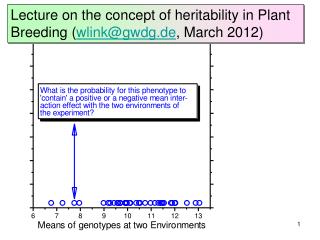
[5] Pi = µ + Gi + (GixE1+ GixE2)/2 positive? negative?
[5] This specific genotype showed an inferior perfor-mance: probably because it is honestly an inferior genotype. Yet, the proba-bility that a (A) negative GxE inter-action contributed to its low performance is larger than the probability that (B) it is genotypically even more inferior and a positive GxE interaction improved its actual performance. Why? Because these ‘even more inferior genotypes’ occur less frequent!
[5] Take the ‘Tour de France’. It is more probable that the winners were doped than the others. Correspondingly, it is more probable that the losers were sick (or suffered from any other specific disadvantage) than the others. Clear?
[5] This specific genotype showed a inferior perfor-mance: probably because it is honestly an inferior genotype. Yet, the proba-bility that a (A) negative GxE inter-action contributed to its low performance is larger than the probability that (B) it is genotypically even more inferior and a positive GxE interaction improved its actual performance. Why? Because these ‘even more inferior genotypes’ occur less frequent!
[5] This specific genotype showed a inferior perfor-mance: probably because it is honestly an inferior genotype. Yet, the proba-bility that a (A) negative GxE inter-action contributed to its low performance is larger than the probability that (B) it is genotypically even more inferior and a positive GxE interaction improved its actual performance. Why? Because these ‘even more inferior genotypes’ occur less frequent!
[5] Significant correlation between results at two locations. r<1 because of GE-interactions Significance of r tells whether r<0, not whether r<1! Diagonal (bisecting line) not really useful here G11+(GE)11.2 The larger the variance due to GE, the smaller is r. I do not know any equation that connects these two parameters.
[5] Effects! Diagonal useful G11+(GE)11.2
[5] Effects! (GE)11.2
[5] With just two environments, (GE)11.2+ (GE)11.7 = 0 Effects!
[5] 13 12 11 10 Means of gentoypes across 12 Envs. r = 0.888** 9 m=0.5789** h²=0.8255 8 7 "E2&E7" 6 6 7 8 9 10 11 12 13 Means of genotypes at two Envs.
[5] The true genotypic values and their estimates from averaging all 12 environments are nearly the same here. The genetic variance is 0.9574