Preliminary Presentation AUV Data Analysis
Preliminary Presentation AUV Data Analysis. MAR 670 Anne-Marie E.G. Brunner. Introduction Data Methods for Project III The Plan Results (final Presentation) Conclusions (final Presentation). 1. Introduction. Turbulence Remus. Upper CTD. Lower CTD. Shear probe FP07 thermistor. ADV.

Preliminary Presentation AUV Data Analysis
E N D
Presentation Transcript
Preliminary PresentationAUV Data Analysis MAR 670 Anne-Marie E.G. Brunner
Introduction • Data • Methods for Project III • The Plan • Results (final Presentation) • Conclusions (final Presentation)
Turbulence Remus Upper CTD Lower CTD Shear probe FP07 thermistor ADV Upward and Down ward ADCPs
*Data have been collected in a passage in Narragansett Bay.*76s of data at a sampling frequency of 1024Hz leads to 77825 data points.*We have measurements of accelerations relative to the bottom – a fixed coordinate system – b1, b2, b3 using an accelerometer.*All three vehicle body accelerations are contaminated by noise mi. The noise is considered to be independent of the other instruments noise.*The water acceleration is measured in y and z with a shear probe relative to the AUV: u1dot, u2dot; these data are also contaminated by noise ni, and again the noise is assumed to be independent of each other and the noise caused by the vehicle acceleration noise.*We further assume, that u1dot and u2dot are not correlated.*A schematic will follow.
All noise is independent of each other and independent of the measured quantities.If the vehicle body accelerations are zero, and all noise is zero, the shear probe would measure the non-contaminated water acceleration.
The three Projects • From acceleration find velocities • The single input case – assume u1dot is only contaminated by b2 and u2dot by b3: Single input – single output. • Assume u2dot is contaminated by b1, b2 and b3: multiple input multiple output.
A short Overview over the Mathematics and Theory The Overall Goal: Determining the decontaminated or corrected Water Acceleration Spectra.
The difference between the estimated and the true spectrum will give the error, dividing this result by the estimated spectrum leads to the delta. The total error is : <delta^2>= random error-biased error= <(delta-<delta>)^2+<delta>^2
“Plan for Project” • Low-pass-filtering of the original data with a cutoff frequency of 32Hz. The Nyquist-frequency is 512Hz. Decimating at half the cutoff frequency (resampling at 128Hz) to reduce the volume of the data (time series contains originally 77825 points) and speed up the calculations. • Applying the filter to a random set of data. • Computing auto-spectra, cross-spectra and co-spectra according to the theory discussed earlier on, especially the decontaminated spectra. • Plot also as variance preserving. • Uncertainty limits • Testing of the Assumptions if possible • Interpretation of results: comparison with the random result, if chance, comparison to SISO results, physical/oceanographic context of results if possible.