Download
1 / 19
250 likes | 591 Vues
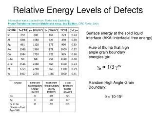
Relative Energy Levels of Defects. Information was extracted from: Porter and Easterling, Phase Transformations in Metals and Alloys , 2nd Edition, CRC Press , 2004. Surface energy at the solid liquid interface (AKA: interfacial free energy).

E N D
Relative Energy Levels of Defects Information was extracted from: Porter and Easterling, Phase Transformations in Metals and Alloys, 2nd Edition,CRC Press, 2004. Surface energy at the solid liquid interface (AKA: interfacial free energy) Rule of thumb that high angle grain boundary energies gb: gb ≈ 1/3 gsv Random High Angle Grain Boundary: q > 10-15o
Processing Using Diffusion 0.5mm 1. Deposit P rich layers on surface. magnified image of a computer chip silicon 2. Heat it. 3. Result: Doped semiconductor regions. light regions: Si atoms light regions: Al atoms silicon • Doping silicon with phosphorus for n-type semiconductors: • Process: Elemental Dot Map from SEM EDS 200X Adapted from chapter-opening photograph, Chapter 18, Callister 7e.
M = mass diffused Jslope time Diffusion • How do we mathematically quantify the amount or rate of mass transfer (rate of diffusion)? • Measured empirically • Make thin film (membrane) of known surface area • Impose concentration gradient • Measure how fast atoms or molecules diffuse through the membrane
C1 C1 C2 x1 x2 C2 x Steady-State Diffusion Rate of diffusion independent of time (does not change with time) • Flux proportional toconcentration gradient = (change in concentration with position) Fick’s first law of diffusion D diffusion coefficient [m2/s] “Diffusivity”
Example: Chemical Protective Clothing (CPC) • Methylene chloride is a common ingredient of paint removers. Besides being an irritant, it also may be absorbed through skin. When using this paint remover, protective gloves should be worn. • If butyl rubber gloves (0.04 cm thick) are used, what is the diffusive flux of methylene chloride through the glove? • Data: • diffusion coefficient in butyl rubber: D = 110x10-8 cm2/s • surface concentrations: C1= 0.44 g/cm3 C2= 0.02 g/cm3
Data: D = 110x10-8 cm2/s C1 = 0.44 g/cm3 C2 = 0.02 g/cm3 x2 – x1 = 0.04 cm Example (cont). • Solution – assuming linear conc. gradient glove C1 paint remover skin C2 x1 x2
æ ö ç ÷ = D Do exp è ø Qd D = diffusion coefficient [m2/s] - Do R T = Material constant [m2/s] Qd = activation energy [J/mol or eV/atom] R = gas constant [8.314 J/mol-K] T = absolute temperature [K] Diffusion and Temperature • Diffusion coefficient increases with increasing T. Arrhenius Equation
What is Do? For Vacancy Diffusion in Cubic Crystal: a is the concentration at jump plane n is the mean frequency of vibration in the jump direction or number of attempted jumps z is the number of available sites to jump to DSm is the activation entropy of migration (increase in entropy due to migration)
T(C) 1500 1000 600 300 10-8 C in g-Fe D (m2/s) C in a-Fe D >> D interstitial substitutional C in a-Fe Al in Al C in g-Fe Fe in a-Fe 10-14 Fe in a-Fe Fe in g-Fe Fe in g-Fe Al in Al 10-20 1000K/T 0.5 1.0 1.5 Diffusion and Temperature D has exponential dependence on T Adapted from Fig. 5.7, Callister 7e. (Date for Fig. 5.7 taken from E.A. Brandes and G.B. Brook (Ed.) Smithells Metals Reference Book, 7th ed., Butterworth-Heinemann, Oxford, 1992.)
transform data ln D D Temp = T 1/T Example: At 300ºC the diffusion coefficient and activation energy for Cu in Si are D(300ºC) = 7.8 x 10⁻¹¹ m2/s Qd = 41.5 kJ/mol What is the diffusion coefficient at 350ºC?
T1 = 273 + 300 = 573K T2 = 273 + 350 = 623K D2 = 15.7 x 10⁻¹¹ m2/s Example (cont.) Note that we have doubled the diffusion rate with 50oC increase in temperature!
Non-steady State Diffusion • The concentration of diffusing species is a function of both time and position C = C(x,t) • The diffusion flux and concentration at a particular point in solid vary with time • Result in net accumulation or depletion of diffusing species Fick’s Second Law: If diffusion coefficient is independent of composition: Solutions to this expression give concentration in terms of both position and time
• Copper diffuses into a bar of aluminum. Surface conc., bar C C of Cu atoms s s pre-existing conc., Co of copper atoms Example Adapted from Fig. 5.5, Callister 7e. B.C. at t = 0, C = Co for 0 x at t > 0, C = CS for x = 0 (const. surf. conc.) C = Co for x =
Solution: C(x,t) = Conc. at point x at time t erf (z) = error function erf(z) values are given in Table 5.1 CS C(x,t) Co
Non-steady State Diffusion • Sample Problem: An FCC iron-carbon alloy initially containing 0.20 wt% C is carburized at an elevated temperature and in an atmosphere that gives a surface carbon concentration constant at 1.0 wt%. If after 49.5 h the concentration of carbon is 0.35 wt% at a position 4.0 mm below the surface, determine the temperature at which the treatment was carried out. • Solution: use Eqn. 5.5
erf(z) = 0.8125 Solution (cont.): • t = 49.5 h x = 4 x 10⁻³ m • Cx = 0.35 wt% Cs = 1.0 wt% • Co = 0.20 wt%
z erf(z) 0.90 0.7970 z 0.8125 0.95 0.8209 Now solve for D Solution (cont.): We must now determine from Table 5.1 the value of z for which the error function is 0.8125. An interpolation is necessary as follows z= 0.93
from Table 5.2, for diffusion of C in FCC Fe Do = 2.3 x 10⁻⁵ m2/s Qd = 148,000 J/mol T = 1300 K = 1027°C Solution (cont.): • To solve for the temperature at which D has above value, we use a rearranged form of Equation (5.9a);
Estimate for Diffusion Distance If you need an engineering estimate for diffusion distance, you can use