THE LAPLACE TRANSFORM
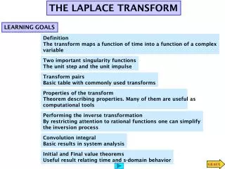
THE LAPLACE TRANSFORM. LEARNING GOALS. Definition The transform maps a function of time into a function of a complex variable. Two important singularity functions The unit step and the unit impulse. Transform pairs Basic table with commonly used transforms. Properties of the transform

THE LAPLACE TRANSFORM
E N D
Presentation Transcript
THE LAPLACE TRANSFORM LEARNING GOALS Definition The transform maps a function of time into a function of a complex variable Two important singularity functions The unit step and the unit impulse Transform pairs Basic table with commonly used transforms Properties of the transform Theorem describing properties. Many of them are useful as computational tools Performing the inverse transformation By restricting attention to rational functions one can simplify the inversion process Convolution integral Basic results in system analysis Initial and Final value theorems Useful result relating time and s-domain behavior
A SUFFICIENT CONDITION FOR EXISTENCE OF LAPLACE TRANSFORM THE INVERSE TRANSFORM Contour integral in the complex plane ONE-SIDED LAPLACE TRANSFORM Evaluating the integrals can be quite time-consuming. For this reason we develop better procedures that apply only to certain useful classes of function
This function has derivative that is zero everywhere except at the origin. We will “define” a derivative for it (Important “test” function in system analysis) Unit step Using square pulses to approximate an arbitrary function Using the unit step to build functions TWO SINGULARITY FUNCTIONS The narrower the pulse the better the approximation
RoC Complex Plane An example of Region of Convergence (RoC) Computing the transform of the unit step To simplify question of RoC: A special class of functions In this case the RoC is at least half a plane. And any linear combination of such signals will also have a RoC that is a half plane
(Good model for impact, lightning, and other well known phenomena) These two conditions are not feasible for “normal” functions Approximations to the impulse Height is proportional to area Representation of the impulse Sifting or sampling property of the impulse Laplace transform THE IMPULSE FUNCTION
LEARNING BY DOING We will develop properties that will permit the determination of a large number of transforms from a small table of transform pairs
Linearity Time shifting Multiplication by exponential Multiplication by time Time truncation Some properties will be proved and used as efficient tools in the computation of Laplace transforms
Homogeneity Additivity APPLICATION Basic Table of Laplace Transforms LEARNING EXAMPLE LINEARITY PROPERTY Follow immediately from the linearity properties of the integral We develop properties that expand the table and allow computation of transforms without using the definition
LEARNING EXAMPLE With a similar use of linearity one shows Additional entries for the table Notice that the unit step is not shown explicitly. Hence LEARNING EXAMPLE Application of Linearity
LEARNING EXAMPLE LEARNING EXAMPLE New entries for the table of transform pairs MULTIPLICATION BY EXPONENTIAL
LEARNING EXAMPLE MULTIPLICATION BY TIME Differentiation under an integral LEARNING BY DOING This result, plus linearity, allows computation of the transform of any polynomial
TIME SHIFTING PROPERTY LEARNING EXAMPLE
LEARNING EXTENSION One can apply the time shifting property if the time variable always appears as it appears in the argument of the step. In this case as t-1 The two properties are only different representations of the same result
Simple, complex conjugate poles Zeros = roots of numerator Poles = roots of denominator Pole with multiplicity r If m<n and the poles are simple PERFORMING THE INVERSE TRANSFORM FACT: Most of the Laplace transforms that we encounter are proper rational functions of the form KNOWN: PARTIAL FRACTION EXPANSION THE INVERSE TRANSFORM OF EACH PARTIAL FRACTION IS IMMEDIATE. WE ONLY NEED TO COMPUTE THE VARIOUS CONSTANTS
LEARNING EXAMPLE “FORM” of the inverse transform SIMPLE POLES Get the inverse of each term and write the final answer Write the partial fraction expansion The step function is necessary to make the function zero for t<0 Determine the coefficients (residues)
USING QUADRATIC FACTORS COMPLEX CONJUGATE POLES Avoids using complex algebra. Must determine the coefficients in different way The two forms are equivalent !
MUST use radians in exponent Using quadratic factors LEARNING EXAMPLE Alternative way to determine coefficients
MULTIPLE POLES The method of identification of coefficients, or even the method of selecting values of s, may provide a convenient alternative for the determination of the residues
Using identification of coefficients LEARNING EXAMPLE
CONVOLUTION INTEGRAL EXAMPLE PROOF Shifting
Using convolution to determine a network response LEARNING EXAMPLE In general convolution is not an efficient approach to determine the output of a system. But it can be a very useful tool in special cases
INITIAL VALUE THEOREM FINAL VALUE THEOREM INITIAL AND FINAL VALUE THEOREMS These results relate behavior of a function in the time domain with the behavior of the Laplace transform in the s-domain
LEARNING EXTENSION Laplace LEARNING EXAMPLE Clearly, f(t) has Laplace transform. And sF(s) -f(0) is also defined. F(s) has one pole at s=0 and the others have negative real part. The final value theorem can be applied.