Control Theory (“Regeltechniek”)
Control Theory (“Regeltechniek”). Jeroen Buijs jeroen.buijs@groept.be Module 7. First example. ROAD. Desired direction. Current direction. Error. Second example. SECOND EXAMPLE:. See http://www.youtube.com/watch?v=8pPfrV8E37o&feature=player_detailpage.

Control Theory (“Regeltechniek”)
E N D
Presentation Transcript
Control Theory (“Regeltechniek”) Jeroen Buijs jeroen.buijs@groept.be Module 7
First example ROAD Desired direction Current direction Error
Second example SECOND EXAMPLE: See http://www.youtube.com/watch?v=8pPfrV8E37o&feature=player_detailpage
Third example – Industrial control ORIGIN OF AUTOMATIC CONTROL 1769: The first automatic controller with feedback in an industrial process Steam engine (James Watt?) Control system (called ‘fly-ball governor’)
Third example – Industrial control ORIGIN OF AUTOMATIC CONTROL Control system: ‘fly-ball governor’
Third example – Industrial control ORIGIN OF AUTOMATIC CONTROL Control system: ‘fly-ball governor’ 1- Turns with speed of output axis of the steam engine. 2- Speed of engine balls towards outside. 3- The movement of the balls regulates the valve of the incoming steam. Balls towards outside Valve closes Less steam speed
History of control theory • In the beginning: based on intuition/heuristics • Second half of 19th century: • Mathematical descriptions (processes => control) • World wars: need for very accurate control systems • (gun positioning, navigation) • the CLASSICAL control period (1914-1960) = design in the frequency domain (Bell laboratories) • 1960-now: MODERN control period • = design in the time domain • Remark: 1969: start of digital control era.
Feedback Example: Thermostatic control PRINCIPLE: 0- Process: Room with in- and outgoing heat flows 1- Measurement: We measure the temperature in the room (T) 2- Comparison: Compare this with the desired temperature (TD) 3- Determine theControl action: If T < TD : Increase heat flow from heating element If T > TD : Decrease heat flow from heating element If T = TD : Don’t change anything 4- Actuate: Use a device to conduct the desired action e.g. increase temperature of water in central heating system Feedback principle:We use a measurement of the output of the process to determine what to do with the input of the process.
Feedback Closed loop / Feedback control system – Block scheme
(No…) Feedback Control system without feedback – Block scheme
Block scheme exercise Block scheme ???
Block scheme of Closed Loop “Servo problem” vs “Control problem”
In practice? Analog PID controllers: Elektronically (4-20mA or 0-10V) Here: for temperature! Pneumatically
In practice? Possible application:
In practice? Desired value 4-20mA Steam flow rate Measured T Typical T-sensor: Pt100 ‘shell and tube’ heat exchanger
Qualitative Analysis Static behavior of the closed loop Servo Problem Control Problem Dynamic behavior of the closed loop
Fext System to be controlled x1,ref x1 Vmot F1 Controller DC Motor (+ transmission) LFJ x2 x2,ref V1 Potentiometer + + V2 Potentiometer + + w2(t) w1(t) Qualitative Analysis
Qualitative Analysis r=zdesired Steady State (SS) error Usually expressed in % zss
Qualitative Analysis x%-settling time Ts,x% Time it takes to get AND keep the signal inbetween x% of the SS value x is typically 2 or 4. Rise time Tr: Time it takes to rise ° [from 0 to 100% of SS value] ° better: from 10% to 90%
Qualitative Analysis Overshoot, usually expressed in %