correlation and percentages
correlation and percentages. association between variables can be explored using counts are high counts of bone needles associated with high counts of end scrapers? similar questions can be asked using percent-standardized data

correlation and percentages
E N D
Presentation Transcript
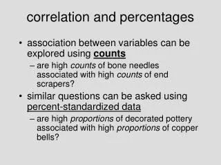
correlation and percentages • association between variables can be explored using counts • are high counts of bone needles associated with high counts of end scrapers? • similar questions can be asked using percent-standardized data • are high proportions of decorated pottery associated with high proportions of copper bells?
but… • these are different questions with different implications for formal regression • percents will show some correlation even if underlying counts do not… • ‘spurious’ correlation (negative) • “closed-sum” effect
10 vars. 5 vars. 3 vars. 2 vars. matrix(round(rnorm(100, 50, 15), nrow=10)))
original counts %s (10 vars.) %s (5 vars.) %s (3 vars.) %s (2 vars.)
original counts %s 10 vars. %s 5 vars. %s 3 vars. %s 2 vars.
including outliers in regression analyses is usually a bad idea… • Tukey-line / least squares discrepancies are good red-flag signals
“convex hull trimming” > hull1 chull(x, y) > plot(x, y) > polygon(x[hull1], y[hull1]) > abline(lm(y[-hull1] ~ x[-hull1]))
transformation • at least two major motivations in regression analysis: • create/improve a linear relationship • correct skewed distribution(s)
LG_DENS log(DENSITY) old.par par(no.readonly = TRUE) plot(DIST, DENSITY, log="y") par(old.par)
transformation summary • correcting left skew: x4 stronger x3 strong x2 mild • correcting right skew: x weak log(x) mild -1/x strong -1/x2 stronger
regression/correlation • the strength of a relationship can be assessed by seeing how knowledge of one variable improves the ability to predict the other
if you ignore x, the best predictor of y will be the mean of all y values (y-bar) • if the y measurements are widely scattered, prediction errors will be greater than if they are close together • we can assess the dispersion of y values around their mean by:
r2= • “coefficient of determination” (r2) • describes the proportion of variation that is “explained” or accounted for by the regression line… • r2=.5 half of the variation is explained by the regression… half of the variation in y is explained by variation in x…
x “explaining variance” range vs.
residuals • vertical deviations of points around the regression • for case i, residual = yi-ŷi [yi-(a+bxi)] • residuals in y should not show patterned variation either with x or y-hat • should be normally distributed around the regression line • residual error should not be autocorrelated (errors/residuals in y are independent…)
residuals may show patterning with respect to other variables… • explore this with a residual scatterplot • ŷ vs. other variables… • are there suggestions of linear or other kinds of relationships? • if r2 < 1, some of the remaining variation may be explainable with reference to other variables
paying close attention to outliers in a residual plot may lead to important insights • e.g.: outlying residuals from quantities of exotic flint ~ distance from quarries • sites with special access though transport routes, political alliances… • residuals from regressions are often the main payoff
Middle Formative, Basin of Mexico
Formative Basin of Mexico • settlement survey • 3 variables recorded from sites: • site size (proxy for population) • amount of arable land in standard “catchment” • productivity index for soils
SIZE (ha) • AGLAND (km2) • PROD (index) How are these variables related? Do any make sense as dependent or independent variables?
(ha) (km2) r2 = .75 y = 35.4 + .66x SIZE = 35.38 + .66*AGLAND
residual SIZE = SIZE – SIZE-hat > resSize frmdat$size – (35.4 +.66 * frmdat$agland)
PROD & SIZE SIZE = -29 + 98 * PROD r2 = .69
r2 = .75 What have we “explained” about site size?? r2 = .69
X0 X1 X2 multiple regression…
X0 1 1 = total variance observed in independent variable (x0)
X0 X1 variance in x0 explained by x1, by itself… variance in x0 unexplained by x1…
X0 X2 variance in x0 explained by x2, by itself… variance in x0 unexplained by x2…
X0 X1 (total variance in x0 explained by x1, that is not explained by x2…) partial correlation coefficient: proportion of variance in x0 explained by x1, that is not explained by x2…
multiple coefficient of determination: variance in x0 explained by x1 and x2, both separately, and together…
productivity agricultural land SITE-SIZE