Download

1 / 40
470 likes | 1.4k Vues
Gravity inversion and isostasy- an integrated system. Trieste, 17-20. February 2003 Carla Braitenberg Dipartimento Scienze della Terra, Università di Trieste, Via Weiss 1, 34100 Trieste Berg@units.it Tel +39-040-5582258 fax +39-040-575519. Topics. Different aspects of isostasy:

E N D
Gravity inversion and isostasy- an integrated system Trieste, 17-20. February 2003 Carla Braitenberg Dipartimento Scienze della Terra, Università di Trieste, Via Weiss 1, 34100 Trieste Berg@units.it Tel +39-040-5582258 fax +39-040-575519
Topics • Different aspects of isostasy: • Local compensation • Regional compensation • Isostasy and sea level change • Examples: • Glacio-isostasy and Hydro-isostasy
Topics • Gravity inversion • Spectral properties of the gravity field • Downward/upward continuation • Iterative inversion procedure • Examples: • Synthetic root • Eastern Alps
Topics • Integration of isostasy and gravity inversion: • Eastern Alps • Tibet plateau • Parana’ Basin • South China Sea
Geographic differences in the MSL variation(Lambeck, Chappell 2001)
Description of geographic differences • Ångermann- river sediments now in 200 m r.p.s.l. • Transgression of sea: change from fresh water to marine sediments • Regression: inverse • Time scale from dating of sediments or counting seasonal Varves • S-England: transition from fresh-water to estuarine deposition • In situ tree-stumps: give upper margin to MSL
Description of geographic differences • Sunda Shelf: flooding of shelf • Barbados: Fossil corals: age-height relation • Dating: Carbon or Uranium series methods • North Queensland: Micro-atoll-formation of corals. Today same corals live in 10 cm depth relative to minimum sea level.
Geographic differences- Description • Classification of observed areas: • Central area of former ice-sheet: Ångermann, Hudson Bay • Marginal areas of ice-sheet or area of small ice-sheets: Åndoya • Medium latitudes, broad area that confined to ice-sheet: South England. The same: Mediterranean, Atlantic coast of SA, Gulf of Mexico. • Areas far from ice-sheet-margin: Barbados, Sunda Shelf • Most observations regard time after LGM: older traces were cancelled by: • A) rising MSL after LGM • B) advancing ice-sheet before LGM
Isostatic Models: locales equilibrium (Airy und Pratt) and regional equilibrium (Flexural Isostasy) • Airy: Variation of crustal thickness as function of topography • Pratt: Variation of crustal density as function of topography
Regional equilibrium (Flexural Isostasy)Model of flexure of a thin plate
Regional equilibrium (Flexural Isostasy) • Flexural rigidity: Typical values: E = 1011 N/m2 = 0.25
Regional equilibrium (Flexural Isostasy) • Insert expressions for p and q: • Solution of equation: k= wave-number We put: We obtain:
Regional equilibrium (Flexural Isostasy) An arbitrary topography can be built as the sum of sine-functions (Fourier-Transormation) The flexure of the plate is then :
Regional equilibrium (Flexural Isostasy) • k= wave-number • W(k)= FT(w(x)) H(k)= FT (h(x)) • To the same result you obtain by applying the Fourier Transformation (FT) of the equation:
Transition to local compensation : With very low flexural rigidity or for small wave-numbers (great wave-lengths) the regional isostasy goes into the Airy Isostasy: With very high rigidity or for small wave-numbers (small wave-lengths) the load does not deform the plate.
Properties of the plate-flexure: • Below the load greatest downward flexure • In the marginal areas: flexural bulge • The smaller the elastic thickness of the plate: • The greater is the amplitude • The smaller is the wave-length of the flexure • At great distances of the load: no effect
Examples • In the simplified Airy case we calculate the subsidence (r) of the crust due to an ice load of thickness (h): Maximum ice-thickness during LGM in scandinavia and North-America estimated to max 2000-2500 m (Lambeck and Chappell, 2001). Gives: r of 600-760 m
Differential sea level change at stable coast and in ocean basin
Examples • In the simplified case of Airy, we calculate the crustal uplift (r) in case of a lowstand of MSL: In occasion of a measured sealevel fall of about 120 m, you obtain r of 40m. The hydro-isostatic effect of MSL-change is then: The comparison with the observations in the Mediterranean shows that the hydro-isostatic effect calculated in the Airy model is over-estimated.
Mean Sea level at the time of the LGM. Lambeck and Bard, 2000
Ice-equivalent sea-level change,from the French Mediterranean area compared to global curves
Ice-equivalent sea-level change,from the French Mediterranean area for late-Holocene time. The continuous curve is same as (i) in (a) (Lambeck and Bard, 2000)
Elastic flexure model:Thin plate approximation Flexure of the crust/lithosphere in frequency space related to topography: Problems in recovering H(k): Low spectral energies in topography Poor spatial resolution caused by required window size in spectral analysis Limitations posed by rectangular window
Convolution method: • spectral domain: • space domain: Flexure point load response Obtained from inverse FT of flexure transfer function Load: refers to total load, being the sum of surface and subsurface load.
Total Load: topographic and buried load Buried load: Lburied inner-crustal loads, hi thickness of the i-th layer, i density of the i-th layer and c the density of the reference crust. Equivalent topography: total load divided by reference density
section across 3D flexure response functions to point load for different flexure parameters
Maximum spatial frequency that must be covered (f0 in 1/km) Sampling (dr in km) Number of elements along the baselength of the square grid (N) Minimum filter extension (Rmax in km) required to reach percentage point 10% and 1% of the maximum value of the impulse response Te f0 (1/km) dr (km) N Rmax (km) Rmax (km) 10% 1% 1 4.00 10-25 500 19 42 2 2.38 10-25 841 33 68 5 1.20 10-210 836 65 135 10 7.11 10-315 938 105 230 20 4.23 10-320 1183 180 400 30 3.12 10-320 1604 245 520 40 2.51 10-330 1326 310 650 50 2.13 10-330 1568 360 760 60 1.85 10-330 1798 400 870
Application of the convolution method in the flexure calculation: • Forward model: given load and Te spatial variation: obtain expected flexure • Inverse model: given load and observed CMI variation: obtain spatial variations of Te
Inverse modeling of Te on synthetic model • Synthetic Moho: created by Paul Wyer with FD solution of loading a spatially varying Te-model with the Eastern Alps topography Resolution: 5 km Size of Moho: 550 km by 500 km • Flexure Moho: • convolution of topographic load with flexure response functions.
On square overlapping windows: for Te=0,...30 km (dTe = 0.5 km) calculate difference between flexure and synthetic Moho Choose Te that minimizes rms Moho Grid: 550km by 500km. Topo: enlarged grid 1200km by 1500 km Te-input model: constant on 15km by 15km cells Moho with noise: noise has rms with 5% of maximal excursion Final Te resolution in space: 30-45 km
Summary isostasy: • Postglacial movements: glacio and hydrostatic movements • flexural isostasy- elastic thickness/flexural rigidity controling parameter • Recover elastic thickness: • convolution method allows high spatial resolution • Inner loads: converted to equivalent topography
References: • Braitenberg, C., Ebbing, J., Götze H.-J. (2002). Inverse modeling of elastic thickness by convolution method - The Eastern Alps as a case example, Earth Planet. Sci. Lett., 202, 387-404. • Lambeck K. , Chappell J. (2001) Sea level change through the last glacial cycle, Science, 292, 679-686 • Lambeck K., E. Bard (2000) Sea-level change along the French Mediterranean coast for the past 30000 years , Earth Planet. Sci. Let., 175, 203-222