
Efficiency & Government Policies
Efficiency & Government Policies. ECON 161 Chapters 7,6. Market Efficiency. Chapter 7. Market Interaction. $ P x. $ 10 $ 9 $ 8 $ 7 $ 6 $ 5 $ 4 $ 3 $ 2 $ 1. Demand. Supply. Pe. Exchange Value. D x. Qty x /T. 1 2 3 4 5 6 7 8 9 10 11 12.

Efficiency & Government Policies
E N D
Presentation Transcript
Efficiency & Government Policies ECON 161 Chapters 7,6
Market Efficiency Chapter 7
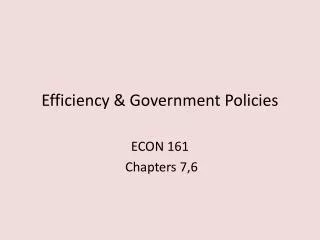
Market Interaction $ P x $ 10 $ 9 $ 8 $ 7 $ 6 $ 5 $ 4 $ 3 $ 2 $ 1 Demand Supply Pe Exchange Value Dx Qtyx /T 1 2 3 4 5 6 7 8 9 10 11 12 Qe
Allocation Efficiency: Price allocates the goods to highest valued users Market Demand determines Price. Each buyer responds to price by buying till Marginal Value equals price. No reallocation can generate greater value. Market A B C $ P Demand Supply $ P $ P $ P D D D Pe Pe Qa Qb Qe Qc Q/T Marginal Value A = Marginal Value B = Marginal Value C = Market Price
Production Efficiency: Price coordinates the efficient use or resources Market Supply is the sum of the industry output at alternative prices. Each firm produces up to the quantity where Price = Marginal Cost. No reallocation of resources will produce at a lower opportunity cost. Market Firm 1 Firm 2 Firm 3 $ P Demand $ P $ P $ P Supply S2 Pe Pe Pe S1 S3 Qe Q/T Q1 Q2 Q3 Market Price = Marginal Cost Firm 1 = Marginal Cost Firm 2 = Marginal Cost Firm 3
Market is Efficient since at Qe the Marginal Value = Marginal cost $ P x $ 10 $ 9 $ 8 $ 7 $ 6 $ 5 $ 4 $ 3 $ 2 $ 1 Demand Supply Pe Dx Marginal Cost Marginal Value Qtyx /T 1 2 3 4 5 6 7 8 9 10 11 12 Qe
Demand = Marginal Value MVx Consumer Surplus Value (MV – Price) $ 10 $ 9 $ 8 $ 7 $ 6 $ 5 $ 4 $ 3 $ 2 $ 1 Pe Exchange Value MVx = Dx 1 2 3 4 5 6 7 8 9 10 Qtyx / T Qe
Supply Reflects Marginal Cost $ P x $ 10 $ 9 $ 8 $ 7 $ 6 $ 5 $ 4 $ 3 $ 2 $ 1 The height reflects the marginal cost of producing an additional unit. Pe Producer Surplus Value Price – Marginal Cost Qtyx /T 1 2 3 4 5 6 7 8 9 10 11 12 Qe
Market: Gains from Trade $ P x $ 10 $ 9 $ 8 $ 7 $ 6 $ 5 $ 4 $ 3 $ 2 $ 1 C.S V. Demand Supply Pe P.S.V. Dx Sx Qtyx /T 1 2 3 4 5 6 7 8 9 10 11 12 Qe
Market Efficiency: Reduced Output $ P x $ 10 $ 9 $ 8 $ 7 $ 6 $ 5 $ 4 $ 3 $ 2 $ 1 Demand Supply Efficiency Loss Pe Dx Sx Qtyx /T 1 2 3 4 5 6 7 8 9 10 11 12 Qe
Market Efficiency:Increased Output $ P x $ 10 $ 9 $ 8 $ 7 $ 6 $ 5 $ 4 $ 3 $ 2 $ 1 Demand Supply Efficiency Loss Pe Dx Sx Qtyx /T 1 2 3 4 5 6 7 8 9 10 11 12 Qe
Market Outcome is Efficient • Marginal Value (MV) of last unit produced = Marginal Cost of production (MC) • Producing less Efficiency loss • Producing more Efficiency Loss
Periods of Analysis • Long-Run: All inputs are variable (prospective) • Short-Run: Some inputs fixed, some variable • Market Period: All inputs Fixed Output Fixed ( vertical supply)
Market Analysis • The Market for Rental apartments • Analyze an increase in demand • Analyze price effects in the market period • Analyze supply and price effects in the long-run
$ Rent Supply LR new Supply D1 D0 New LR Equilibrium $ 1000 $ 880 $ 800 Units/Month 1000 1500
$ Rent Supply D0 Price Ceiling $ 800 D1 Short Units/Month 1000 1500
Implications Price Ceiling below Equilibrium • Increased Transaction Costs to Buyers & Sellers • Increase in Non-Market rationing: Discrimination • Decrease in Quality • Decrease in Supply
Price Floor above Equilibrium • How does the labor Market work? • What happens when you place the Minimum Wage above Equilibrium wage ?
$ Wage Supply of Labor Demand Min. Wage Wage E Surplus Qty/T Qd QE Qs
The Minimum Wage: A Price Floor $Wage D S Minimum Wage Pe D Qd Qe Qs QTY / T
Implications of Price Floor above Equilibrium • Increase in transaction costs • Increase in non-market rationing (discrimination) • Increase in quality (not demand driven) • Increase in supply • Wealth transfer: from unemployed to employed
Sales Tax on Buyers Sx $ Price x $Pb $Pe Tax Revenue $Ps Dx Dx’ Qt Qe Qty x /T
Tax on Sellers Sx’ $ Price x Sx $Pb $Pe Tax Revenue $Ps Dx Qt Qe Qty x /T
Tax Burden: Inelastic Demand $ Price x $Pb Sx $Pe Tax $Ps Dx Qt Qe Qty x /T
Tax Burden: Inelastic Supply Sx $ Price x $Pb $Pe Tax $Ps Dx Qt Qe Qty x /T